
PineconeX Documentation
Version: v0.2.2-alpha
PineconeX is a SaaS platform for backtesting and live-trading Pine Script® v6 strategies against real market data. Write your strategy once, then backtest it, sweep its parameters, validate that the edge is real, and deploy it live against a connected broker, all from the same interface.
Equities and crypto. Alongside European and US stocks, PineconeX trades crypto: USD and EUR spot pairs on Bitstamp, the US-dollar pairs on Alpaca, and the USDT pairs on Binance. Crypto markets never close, and the venues' order models differ from an equity broker's in ways that change how a stop-loss behaves, so read this before deploying a crypto bot.
Table of Contents
- Getting started
- Strategies
- Backtest
- Debugging with log.info()
- Parameter Sweep
- Validation
- Machine Learning Models
- Gamma Exposure (GEX)
- Basket readings (
basket.*) - Volume Profile (vp.*)
- Live Trading
- Tick data vs. bar data
- Sentiment and attention
- Market Data
- What a bar contains (OHLCV)
- What a strategy knows about its instrument (syminfo.*)
- Buying and selling volume (volume delta)
- Price structure: what the market did before your strategy
- Supported sources
- Data quality: what is checked when data is fetched
- Reading another symbol (request.security)
- Company fundamentals (ESEF:)
- Futures
- Brokers
- Plans
Getting started
Sign in at pineconex.com with your Google account. No separate registration is required.
Tip: We recommend signing in with your GitHub account, which enables seamless version management of your strategies directly from your repositories.
On first login you are placed on the Free plan. A free trial period gives you temporary access to Pro features so you can explore the platform before committing.
Strategies
The Strategies page is your library of Pine Script v6 strategies. Each strategy has a Monaco-based code editor with Pine Script syntax highlighting and an inline validator that catches errors before you submit a job.
Learning Pine Script v6
PineconeX runs standard Pine Script v6, so the official TradingView documentation is your primary language reference:
- Pine Script v6 User Manual. The language guide: syntax, types, execution model, and how-to tutorials.
- Pine Script v6 Reference Manual. The full API reference for every built-in function, variable, and keyword (
ta.*,strategy.*,str.*, …). - TradingView Community Scripts. Thousands of published open-source strategies and indicators to learn from and adapt.
For the trading side rather than the language, the Learn hub collects the books, talks and guides we recommend on systematic trading, backtesting and validation.
v6 only. A community script written for v4 or v5 is refused here, and most published scripts still are. If you have a TradingView account, its Pine Editor will convert one for you (open the script, then Convert code to v6), and that is the fastest route. Otherwise change
//@version=5to//@version=6and re-validate: the validator reads your source and names the specific constructs in it that v6 removed, with what to write instead, so you fix the lines it lists rather than reading a migration guide end to end. Two changes have nothing to grep for and are always mentioned:margin_longandmargin_shortdefault to 100 in v6 where they were 0 in v5 (so an implicitly leveraged strategy reports different numbers), and aboolcan no longer holdna.
PineconeX runs Pine headless. There is no chart, so chart/UI calls (
plot,hline, drawings, tables, …) are accepted but silently ignored, and a few primitives diverge from TradingView (e.g.alertcondition()is repurposed for notifications). The language is the same; the runtime is backtest/live execution rather than a chart. These differences are called out throughout this guide where they matter.
Creating a strategy
- Click New strategy.
- Give it a name and paste or write your Pine Script v6
strategy()code, or start from one of the templates in the picker. - Click Validate to check for syntax errors.
- Save. The strategy is now available in the Backtest, Sweep, Validation, and Live launchers.
A template's tier is the tier its dependencies already sit behind, not a pricing choice, and it is computed from the file rather than declared: the templates marked Premium read a second timeframe off their own symbol or need a trained model, and the two marked Pro document a Pro-only live feature (a webhook URL, Telegram notifications). Selling one below what it needs would be a door onto a wall, where the strategy is created and then refused on the one thing it was written to do.
Importing from GitHub
Link your GitHub account under Account → GitHub, then use Import from GitHub to pull any .pine file from your linked repository. Imported strategies stay in sync: changes pushed to GitHub are reflected automatically. GitHub-imported strategies do not count against your strategy quota.
Sharing a strategy
Open a strategy and click the Share button. You can make it:
- Private: only you can see it.
- Open: anyone with the link gets a private, editable copy of the strategy added to their own account (a fork). They get the full code, but as their own copy, and your original is untouched.
- Protected: link required plus you grant access per user. Granted users can run backtests and live bots with the strategy, but the source code stays private: it is never shown to them. The strategy is shared; the code is not.
Write-protected strategies
A strategy is locked against editing while a live bot is running it, or while it is held in your fleet snapshot. The tile shows a Write-protected badge, the editor opens read-only, and Save is replaced by an explanation. Validate still works, since reading and checking a file is always safe.
The reason is not caution, it is that editing would not do what it looks like it does. A bot runs the code it was launched with. The source is copied into the bot when it starts and is never re-read, so editing the file under a running bot cannot change what is trading. All it would do is make the file disagree with the account, on the very page you would look at to find out what a bot is running.
The snapshot extends the same protection forward in time. Restore relaunches from the file as it reads then, so an edit made while the bots are down would change what Restore starts, and the snapshot would name one fleet and start another.
The .pine and its .json5 lock together, because a bot froze both when it launched.
To edit a locked strategy, stop the bot, or save a new snapshot that does not include it. If you want to try changes while a bot keeps running, copy the strategy and edit the copy.
This applies to strategies hosted on PineconeX. A strategy imported from GitHub is already read-only here, and its real file lives in your repository, where this platform cannot protect it.
Alongside the badge, each tile shows either a live indicator (how many bots are running it right now) or the date it last ran live, never both.
Parameter overrides (JSON5)
For each strategy you can define parameter overrides in JSON5 format via the Params editor. This lets you store a set of symbol/timeframe combinations with their tuned input values, so jobs pick them up automatically without editing the Pine source.
Format:
[
  {
    symbol: "AAPL",
    configs: [
      { tf: "1D", htf: "1W", ltf: "60m", length: 20, threshold: 0.5 },
      { tf: "60m", length: 10 }
    ]
  }
]
symbol, tf, htf, and ltf are reserved keys; every other key must match the variable name of one of your input.*() calls. The Params editor validates them against the parsed inputs in real time.
tf: the primary bar resolution for that config.htf: optional higher timeframe (forrequest.security). On the Backtest form it pre-selects the higher-timeframe dataset; on live bots it maps to your strategy'shtfinput.ltf: optional lower / intrabar timeframe (forrequest.security_lower_tf). On the Backtest form it pre-selects the Intrabar TF dataset; on a live bot it sets the intrabar warmup resolution fetched from the broker feed. (Sweep supports intrabar too, but picks it from its own form control rather than from this key. The Significance test rejects an intrabar series, see Validation.)
All three timeframe keys accept the same timeframe strings as the pickers.
Timeframe syntax
Timeframes use a uniform, minute-based notation everywhere in PineconeX (the Params JSON5, the Data catalog, and the Backtest / Sweep / Validation / Live pickers). Use these exact strings; they are case-sensitive:
| String | Resolution |
|---|---|
1m | 1 minute |
5m | 5 minutes |
15m | 15 minutes |
30m | 30 minutes |
60m | 1 hour |
90m | 90 minutes |
1D | Daily |
1W | Weekly |
1M | Monthly |
Intraday resolutions are written in minutes (<n>m); daily and above use 1D / 1W / 1M. The legacy 1H (= 60m) and 4H (= 240m) aliases are still accepted for backward compatibility, but prefer the minute form.
Live bots trade the broker feed directly (no stored dataset), so they omit weekly/monthly and the 1-minute step. The available live timeframes are
5m,15m,30m,60m,90m,1D. Keep a config'stfwithin this set if you plan to run it live.
Trading costs & fill realism
The engine simulates the standard Pine Script v6 strategy() cost and fill-assumption arguments, so your backtests can reflect real-world frictions. These apply to Backtest, Parameter Sweep, and Validation runs (live bots submit real orders instead):
| Argument | Effect |
|---|---|
commission_type + commission_value | Per-trade commission, charged on both legs. Three modes: strategy.commission.percent (% of each fill's value), strategy.commission.cash_per_contract (fixed cash per share/contract), and strategy.commission.cash_per_order (flat cash per order). |
slippage | Worsens the fill price of every market and stop order by a number of ticks (0.01 price units): buys fill higher, sells fill lower. Limit / take-profit fills are exempt. |
backtest_fill_limits_assumption | Models unfilled limit orders: a limit (take-profit) order only fills after price moves this many ticks past its price, instead of the moment price touches it. |
All default to no cost (0), so a strategy without these arguments backtests frictionlessly. See the inline comments in the default strategy template for exact syntax.
Same-bar stop and target (the bar magnifier)
When one bar's range touches both a resting stop and a resting take-profit, the bar's four prices cannot say which one price reached first. The engine's default is to book the take-profit, which is optimistic and flatters every bracket strategy.
strategy(use_bar_magnifier = true) resolves those ties from finer data instead:
| Where | How a tie is resolved |
|---|---|
| Backtest and Sweep | The engine walks the Intrabar (LTF) sub-bars inside the ambiguous bar and books whichever leg price actually reached first. A single sub-bar that touches both legs is itself ambiguous, so the stop wins there. If no sub-bar covers the bar, it falls back to the optimistic default rather than inventing a worse result from missing data. |
| Significance and Stress | The permutation null rebuilds every bar, so real sub-bars cannot apply. The tie is resolved from the recomposed bar's own OHLC with a driftless Brownian bridge, P(low before high) = (high − open) / (high − low), booking the more likely leg first, with an exact 50/50 breaking to the stop. Deterministic on purpose: the only randomness stays the seeded shuffle, so the p-value remains reproducible. |
- In a backtest or sweep the flag needs an intrabar series. Without one it is a silent no-op (a warning appears in the log). Pick an Intrabar TF on the form, or set
ltfin your JSON5 params. Validation needs no series; it resolves ties from the bar itself. - It is opt-in and inert by default. A strategy without the flag produces byte-identical results to before.
- Expect the numbers to get worse when you switch it on. That is the point. On real 15-minute sub-bars under a 1-hour chart, a bracket strategy moved from a 62% win rate and 1.70 profit factor to 55% and 1.28. Nothing was lost; the optimistic bias was removed.
Position sizing
By default a strategy trades one share/contract per order. Control the order size with the standard Pine Script v6 strategy() arguments default_qty_type and default_qty_value:
default_qty_type | Order size |
|---|---|
strategy.fixed | Exactly default_qty_value shares/contracts. |
strategy.cash | As many whole shares as default_qty_value (in account currency) buys: floor(value / price). |
strategy.percent_of_equity | A position worth default_qty_value % of account equity: floor(equity × value / 100 / price). |
strategy("My strategy", default_qty_type = strategy.percent_of_equity, default_qty_value = 10)
What to know about live bots:
- Whole shares only. Equity orders are rounded down to whole shares; if the computed size is below one share the order is skipped. (Crypto keeps fractional size.) Because of the round-down, a
cashorpercent_of_equityorder usually deploys slightly less than the nominal amount: $5,000 of a $294 stock buys 16 shares (≈ $4,714), not a fractional 16.9. percent_of_equityuses your real broker equity. A live bot reads your connected account's current equity to size the order and refreshes it as the account value changes. Backtest, sweep, and validation runs use the strategy'sinitial_capitalinstead.
Sizing each order from the market's current volatility, instead of a fixed cash or equity fraction, is a separate feature: see Basket readings (
basket.*).
Margin and leverage (margin_long / margin_short)
Both default to 100, meaning full cash cover and no leverage, exactly as Pine Script v6 does, and an entry that would need more money than the account has is not opened. So default_qty_type = strategy.percent_of_equity, default_qty_value = 400 no longer quietly borrows four times your equity; it is capped at what you can actually pay for.
If you want leverage, say so: strategy(..., margin_long = 25) is 4× (25% of the position value must be covered). An explicit margin_long = 0 also maps to 100 rather than to "unlimited", because reading a 0% requirement literally would mean infinite leverage, which is the most dangerous possible interpretation.
This changes historical backtest numbers. A strategy that was implicitly over-leveraging now reports lower, realistic results, because the entries it could not afford are no longer taken. TradingView would not have taken them either, and that is what makes a PineconeX backtest and a TradingView backtest of the same script agree.
Our margin limit is not your broker's. It never goes over the wire: an order carries only a quantity, and your broker applies its own Reg T / maintenance rules independently. The two never talk, which is exactly why ours must not be looser than theirs. On a live bot, see Margin monitoring.
Pyramiding
strategy(pyramiding = N) caps how many entries may be added in the same direction while a position is open. The default, pyramiding = 0, allows a single entry, so additional same-direction entry signals are ignored until the position is closed. A reversal (an opposite-direction entry) is always allowed.
Entries stack: with pyramiding = 3, three same-direction entries build one larger position and the fourth is refused until the position closes. It works the same way in a backtest, a sweep and a live bot.
Each entry is sized in full.
default_qty_value = 25withpyramiding = 4commits 100% of equity, not 25% split four ways. Size for the stack you intend to hold rather than for one entry.
Stacked entries close as one trade. PineconeX holds a single netted position rather than a list of individual entries, so three stacked entries exit together, as one trade at their size-weighted average price. TradingView unwinds each entry separately. The total profit and loss agrees; the trade list and the trade count do not. That is also why
close_entries_rule(FIFO vs ANY) has nothing to decide here, and is accepted and ignored.
A pyramiding entry must be a market order. A resting
limit=orstop=entry cannot be added to a position that is already open, because a resting order cannot be matched against the position it would join. In a backtest such an order rests until it fills or expires; a live bot refuses it and says so in the job log.
Results recorded before 2026-08-18 were measured without this.
pyramidingwas read and then had no effect, so a strategy setting it above0traded a single lot. If you have numbers for such a strategy from before that date, re-run it: the old figures describe a smaller system. Strategies left at the default0are unaffected and their numbers stand.
Resizing a position (strategy.order)
strategy.order(id, direction, qty = n) changes the size of a position that is already open, and unlike strategy.entry it ignores pyramiding entirely. It is how a strategy rebalances: volatility targeting, risk parity, rebalancing bands, and Kelly sizing all hold one position and adjust it as their estimate moves.
Three cases, and the accounting differs in each:
| the order is | what happens |
|---|---|
| the same direction | the position grows, and its cost basis becomes the size-weighted average of the old basis and this fill |
| opposite, smaller | the position shrinks. The closed part books a real trade at the original basis; what remains keeps that basis, because selling part of a holding does not change what the rest cost |
| opposite, larger | the position closes and the surplus opens the other way, as TradingView does |
A reverse is refused where the venue cannot hold a short. Bitstamp spot and Alpaca crypto are long only, so the closing part is placed and the surplus is refused rather than sent. The bot ends flat, and says so in the job log. Alpaca equities can hold a short, and the bot asks your account whether it may before opening one.
Results recorded before 2026-08-18 were measured without this too.
strategy.orderwas accepted and did nothing at all, with no error and no log line, so a rebalancing strategy sized its position once and then held it unchanged. The tell is a strategy that reports one trade whose return equals the instrument's own price move.
History buffer (max_bars_back)
strategy(max_bars_back = N) sets how many past bars the engine keeps so your code can reference earlier values of a variable (myVar[n]). Omit it and PineconeX auto-sizes the buffer to the deepest [n] lookback in your code, just like TradingView, so you never pay for history you don't reference.
Set it explicitly (0–5000) only when the depth can't be known ahead of time, e.g. a variable indexed by a loop counter or another series (myVar[i]). Then give the engine an upper bound, exactly as TradingView asks you to.
Built-in series (
close[n], …) andta.*functions always see full history regardless of this setting; it only bounds user-variable lookback.
Indexing a past value behaves as it does on TradingView:
ta.rsi(close, 14)[1],(close > open)[1],math.sum(close, 5)[1],close[1][1],(cond ? a : b)[1],strategy.equity[1]andta.obv[1]all work, andexpr[0]is always the expression itself. Four things refuse, each with a clear error rather than a wrong number: a tuple at a non-zero offset (ta.macd(...)[1]— destructure it first with[m, s, h] = ta.macd(...), which is how TradingView works too),barstate.*/session.*, a user-defined function whose body is just a bool or a number, andtimeframe.change(). Assigning to a variable first and indexing that (e = ta.ema(close, 20)thene[1]) fixes all four and is never wrong. Engines before2026.08.29-zeroindexindex only part of the surface and raise an error for the rest, so pin that version or newer if you rely on it.
Ending a run early (runtime.exit)
runtime.exit("reason") stops the run and records why.
It is not the same as runtime.error(). An error means something went wrong on this bar, and
every engine skips that bar and carries on, so a strategy cannot stop itself with one.
runtime.exit means there is nothing more for me to do, and the run ends.
//@version=6
//@runtime=2026.09.05-runtimeexit
strategy("Stops itself", overlay = true)

// A model fitted to one regime should not keep trading once the regime is gone.
if ta.atr(20) > ta.atr(200) * 3
    runtime.exit("volatility left the range this strategy was fitted on")

if ta.crossover(close, ta.sma(close, 20))
    strategy.entry("L", strategy.long)
Needs engine
2026.09.05-runtimeexitor newer. On an older engine the script does not merely ignore the call, it fails to compile:Type error: Object has no member 'exit'. Pin the version as above, or leave the strategy unpinned to get the current default.
It works in every run type, and each one ends the thing it owns:
| Run type | What stops |
|---|---|
| Backtest | No further bars are processed. The run finalizes exactly as it does when the data runs out, and every statistic is computed over the bars that ran. |
| Parameter sweep | Only the trial that called it. That trial is still scored, on the bars it ran, and still appears in the surface. |
| Significance / stress | Same as a sweep: the run that called it ends, the rest of the permutations continue. |
| Portfolio backtest | Only the leg that called it. The book keeps running with the remaining legs. |
| Live bot | The bot cancels the orders it left resting at your broker, then exits cleanly. |
Where the reason turns up
The reason is the point of the feature, and it is recorded in three places so a run that stopped early never gets mistaken for one that crashed or one that quietly ran out of data:
| Where | What you see |
|---|---|
| Job log | runtime.exit — the strategy ended the run at bar 300 of 7232: <your reason> |
results.json | summary.exit_reason, which is null on every run that was not stopped by the script |
| Bot history (live bots) | an exit event with your reason in the Detail column |
That last row is a separate event type on purpose. stopped means a person pressed stop, crashed
means the container failed, and exit means the strategy decided. Reading a bot's history, those
are three different stories and they should not share a heading.
A sweep announces it once per run, not once per trial. A swept axis that trips the exit condition trips it in many cells at once, and a line for each would bury the surface you are reading.
Five things to know
-
The bar that calls it still finishes. Everything after the
runtime.exitline runs, and any order that bar placed is kept. Only the bars after it are skipped, so nothing you had already committed to on that bar is thrown away. -
A live bot does not close your positions. It cancels resting orders, because an order with no bot behind it is a hazard, and it leaves any open position alone and names it in the log, because a position is an asset you still own. To close it as well, close it in the strategy first, or use Stop and flatten from the job page.
-
A live bot ignores it during warmup. A bot replays historical bars to warm its indicators before it trades. A condition that was true somewhere back in that history would otherwise stop the bot before it ever placed an order, so requests made during the replay are dropped.
-
Do not trigger a live bot on
bar_index. Because of that replay, the index at the first live bar depends on how much history the bot loaded and is not knowable when you launch it. Count real-time bars instead:var int live_bars = 0 if barstate.isrealtime live_bars := live_bars + 1 -
It is not TradingView portable. TradingView has no
runtime.exit, so a strategy using it will not compile there.runtime.error()exists on both, but it does not do the same thing.
A bare runtime.exit() stops the run just the same, but the reason is what makes a job log readable
weeks later, so it is worth writing one.
Time zones and sessions
Every bar is stamped in UTC, and the bare hour, minute, dayofweek and dayofmonth
variables read that stamp. TradingView reports them in the exchange's own time, so this is a real
difference and it is silent: a gate written as hour == 9 is a 09:00 UTC gate here, which on a
US equity is four or five hours before the open depending on the month.
The fix is not to shift the variable. It is to ask for the time zone you mean:
inRTH  = not na(time(timeframe.period, "0930-1600", "America/New_York"))
nyHour = hour(time, "America/New_York")
gate   = timestamp("America/New_York", 2024, 1, 2, 9, 30)
| form | what the time zone does |
|---|---|
time(tf, session, tz) | reads the session window on that zone's wall clock, and returns na outside it |
hour(t, tz), minute(t, tz), dayofweek(t, tz), dayofmonth(t, tz), month(t, tz), year(t, tz) | converts the instant before splitting it, so the day can change as well as the hour |
timestamp(tz, year, month, day, hour, minute) | reads the components as a local wall clock in that zone, not as UTC |
str.format_time(t, format, tz) | formats the stamp on that zone's clock, so the printed date can differ from the UTC one |
Both spellings are accepted: an IANA name ("America/New_York", "Europe/London", "Asia/Tokyo")
or a fixed offset ("UTC+2", "GMT-5", "+02:00").
Prefer the name. A fixed offset is frozen, so "UTC-5" is New York in January and an hour wrong
from March to November. A name carries the transition dates, including the ones that have since
changed: US daylight saving moved in 2007 (it used to begin in April, it now begins in March), and
Moscow left daylight saving entirely in 2011. Backtests here routinely run over decades, so a frozen
offset is wrong for a large part of the history it is applied to, on every intraday bar, without
failing.
A name that does not exist is refused, not quietly treated as UTC. The names are case-sensitive and use an underscore, so
"America/New York"and"america/new_york"are both errors. That is deliberate: a session an hour out produces numbers that look entirely reasonable.
Older engines did not do any of this.
time()refused every named zone outright, whiletimestamp(),hour()andstr.format_time()accepted one and ignored it, returning the UTC answer under the name you had asked to convert. If a strategy of yours computes daylight saving by hand to work around that, you can delete the arithmetic and pass the name.
Asking the instrument instead of naming a zone
syminfo.timezone answers with the listing exchange's zone, so the TradingView idiom works
unchanged and a strategy stays portable across instruments:
inRTH = not na(time(timeframe.period, "0930-1600", syminfo.timezone))
That reads the New York session on a US listing and the Frankfurt session on a German one, from the
same source line. 98% of the catalog carries a zone; the exceptions are the rows that have no
exchange at all (WIKI: pageviews, ESEF: fundamentals, SECFORM4:, CNN:), and those answer
"UTC".
This changed on 2026-09-03, and it changes results.
syminfo.timezonewas the string"UTC"on every instrument before that date, so any strategy passing it totime()ortimestamp()was gating on a UTC window rather than the exchange's. Nothing failed and nothing warned: the script ran, traded, and reported plausible numbers on the wrong hours. If you have figures for such a strategy from before that date, re-measure them. The strategy now does what its source reads as doing, which on a US listing is a window four or five hours from where it actually sat.
time_close(timeframe, session, timezone) takes the same three arguments as time() and returns
the period's closing stamp rather than its open. The bare time_close variable is a different
thing and keeps its own meaning: the close time of the current bar.
Backtest
Run a single backtest of a strategy against a historical dataset.
Configuration
| Field | Description |
|---|---|
| Strategy | Select a strategy from your library. |
| Symbol / Index | Pick the market index, then the individual symbol. |
| Timeframe | Bar resolution for the primary series (1M, 1W, 1D, 90m, 60m, 30m, 15m, 5m, 1m). See Timeframe syntax. |
| Higher timeframe | Optional. The request.security series. Pre-fillable from the htf key in your JSON5 params. |
| Intrabar TF | Optional. The request.security_lower_tf (intrabar) series. Pre-fillable from the ltf key in your JSON5 params. Also the series use_bar_magnifier resolves same-bar stop/target ties from. Without it, the flag does nothing. |
| Date range | Start and end date for the historical window. |
| Data source | Which feed the bars come from: Yahoo, Saxo, Alpaca, Bitstamp, Massive or IBKR. Only the sources that actually carry the selected symbol are offered. See Supported sources. |
Results
Once the job completes, the results page shows:
- Equity curve: cumulative net profit over the backtest period.
- Drawdown: underwater equity plotted over time.
- Trade list: every entry and exit with date, price, P&L, and run-up / drawdown.
- Metrics: net profit, gross profit/loss, max drawdown, Sharpe ratio, win rate, profit factor, average trade, number of trades, and more.
- Logs: raw container output for debugging.
- AI analysis: optional one-click AI narrative summarising performance (requires a configured AI provider).
The report used to carry a Data block (Hurst, variance ratio, price structure). It has moved to the Data page's Structure tab, because it described the price series, so it was identical for every strategy ever run on that dataset, the same three numbers on every winner and every loser, sitting next to figures that really were the strategy's.
Comparing backtests
Select up to 5 completed backtests from the history list using the checkboxes, then click Compare. The comparison view overlays equity curves and places metrics side by side for easy evaluation.
Debugging with log.info()
When a strategy isn't trading the way you expect, the fastest way to see why is to print the values your logic depends on. PineconeX supports the standard Pine Script v6 logging functions:
| Function | Use for |
|---|---|
log.info(msg) | General trace output: values, flags, "did this branch run?" |
log.warning(msg) | Something unusual but non-fatal. |
log.error(msg) | A condition your strategy treats as a hard problem. |
Each message shows up in the run's Logs panel (Backtest, Sweep, and Validation results all have one), and streams live in a bot's Logs view for live trading. In a backtest each line is prefixed with the bar timestamp it was emitted on, so you can line the output up against the chart.
Printing values
log.* takes a single string argument, so to print a number, a boolean, or a series value you convert it with str.tostring() and join the pieces with +:
//@version=6
strategy("Debug demo", overlay = true)

fast = ta.ema(close, 10)
slow = ta.ema(close, 30)
cross_up = ta.crossover(fast, slow)

// Print the values every bar
log.info("close=" + str.tostring(close) + " fast=" + str.tostring(fast, "0.00") + " slow=" + str.tostring(slow, "0.00") + " cross_up=" + str.tostring(cross_up))

if cross_up
    strategy.entry("Long", strategy.long)
    log.info("ENTRY long @ " + str.tostring(close, "0.00"))
A few things to know:
str.tostring(value, "0.00")applies a format string, here two decimal places. Handy for prices and indicator values that would otherwise print a long float.- Booleans and
naprint directly.str.tostring(cross_up)givestrue/false, and anavalue prints asna, so you can see exactly when a value is missing. - Series and
ta.*results log their current-bar value automatically. You don't need to index them:str.tostring(ta.rsi(close, 14))prints this bar's RSI. (To inspect a past value:str.tostring(ta.rsi(close, 14)[1]), or assign it to a variable first and index that — see the note on indexing indicator values.) - No
{0}placeholders. Unlike TradingView, PineconeX does not support format-placeholder logging (log.info("x={0}", x)); only the first argument is read, so build the whole string with+.
Tracing why a signal did or didn't fire
The most useful pattern is logging the individual conditions that gate an entry, so you can see which one is blocking:
long_ok = cross_up and close > slow and strategy.position_size == 0

if ta.crossover(fast, slow)
    log.info("cross seen | above_slow=" + str.tostring(close > slow) + " flat=" + str.tostring(strategy.position_size == 0) + " -> entry=" + str.tostring(long_ok))
Now every time the EMAs cross you get one line showing exactly which guard passed or failed, far quicker than guessing.
Keep the log readable
Logging every bar floods the panel and (for live bots) counts against the captured-log size cap. Gate your debug output behind the condition you actually care about so you only print on the interesting bars:
// Only log around a potential signal, not on every bar
if cross_up or cross_down
    log.info("signal bar: " + str.tostring(close, "0.00"))
Tip: Leave the
log.*calls gated behind aninput.bool(false, "Debug")toggle so you can flip verbose tracing on and off without editing the strategy:debug = input.bool(false, "Debug logging") if debug log.info("state: " + str.tostring(myVar))
Parameter Sweep
Systematically search the parameter space of a strategy to find robust configurations.
Sweep annotation
Mark which inputs to sweep by adding //@sweep before their input.*() call:
//@sweep
fast = input.int(10, minval=2, maxval=50)
//@sweep
slow = input.int(30, minval=10, maxval=200)
PineconeX reads the minval and maxval from each annotated input to define the search bounds automatically.
Sweep modes
| Mode | Description |
|---|---|
| RBF Optimise | Cubic RBF surrogate model. Fewest evaluations needed; smart interpolation between sample points. The only mode that steers: it hill-climbs the chosen objective. Based on Costa & Nannicini, RBFOpt (2016). |
| Grid | Exhaustive 2-D grid over the two swept parameters. Best when you need to see the full landscape. |
| Random | Uniform random sampling across all swept parameters. Fast, unbiased exploration. |
Objective
The steering mode (RBF Optimise) hill-climbs a single number, the objective. Grid and Random don't steer, so they have no objective: they emit every trial and you rank the results afterwards by any metric.
Built-in objectives: net_pnl_pct (default), return_over_dd, sharpe, profit_factor,
expectancy, win_rate, and max_dd_pct (minimised).
Custom expression. Pick Custom expression… to write your own objective as an arithmetic formula over the trial metrics, for example:
net_pnl_pct - 0.5 * max_dd_pct + 0.1 * trades
- Variables:
net_pnl_pct,max_dd_pct,trades,win_rate,profit_factor,expectancy,sharpe,return_over_dd. Operators:+ - * / ( )and numbers. - The search maximises the expression as written, so a penalty term gets a minus sign.
max_dd_pctis a positive percentage (a 12% drawdown is12), so subtract it to punish risk. - A trial below the Min trades floor can never win, custom objectives included, because otherwise a
config that barely trades can score arbitrarily well (a division by zero, e.g. a zero-drawdown
fluke in
pnl / dd, is also disqualified rather than winning by infinity).
Results
- Heatmap: net profit (or any metric) plotted as a colour grid over the two swept parameters. Reveals whether good performance is isolated (fragile) or spread across a region (robust).
- Ranked runs: all completed trials sorted by the chosen metric. Click any row to drill into that run's full backtest results.
Time limits
Sweeps and backtests run under a maximum wall-clock time. A job that exceeds its limit is stopped automatically and marked failed, so a very large grid or a long date range may need to be narrowed to finish in time. Live bots are not time-limited.
Validation
A backtest tells you what happened. Validation asks whether to believe it.
Both tests place your result against a distribution the strategy was not fitted to, and that is what separates them from a backtest with different settings. Premium plan.
Significance: is the edge real, or luck?
The price series is bar-permuted hundreds of times: each bar is decomposed into its gap and its intrabar moves, those are shuffled independently, and valid OHLC bars are rebuilt. The result keeps the return distribution and the candle geometry but destroys the cross-bar sequence, the very thing a strategy claims to exploit.
Your strategy is then run against every one of those scrambled series. If it only made money because it happened to catch real moves in the real order, it will fall apart on them. If it keeps making money on scrambled prices, it was never reading the market. It was reading the return distribution, which any rule can do.
The headline number is how often the scrambled series did as well as or better than the real one. Two out of two hundred means your result is hard to get by luck. Ninety out of two hundred means it is not.
| Field | Description |
|---|---|
| Permutations | How many scrambled series to test against (default 200). More is finer-grained: with only 50, the best result you can possibly report is "1 in 51". |
| Test statistic | What counts as "doing well": Net P&L % (default), Return / drawdown, Sharpe, Profit factor, Expectancy, Win rate, or a custom expression over the trial metrics (same syntax as the Sweep objective, e.g. net_pnl_pct - 0.5 * max_dd_pct). It is both the reported statistic and, for a searching procedure, the objective the search hill-climbs inside every permutation. |
| Permutation type | Bar scrambles every bar independently, the strictest test. Block shuffles chunks of N bars, keeping short-term patterns intact. Use Block if your edge is meant to play out over days rather than bars. |
| Where the settings came from | The most important control on the page. See below. |
| Seed | Leave empty for a random run. The seed used is reported back, so any run can be reproduced exactly. |
If you found your settings with a Sweep, say so
This is the one setting that can quietly invalidate the whole test.
Fixed params (the default) runs your strategy with the numbers written into the script, exactly as they are, on every shuffled series. That is the right test if you chose those numbers yourself, from theory, from a book, from experience.
It is the wrong test if you found them with a Sweep.
Here is why. A Sweep tries many combinations and hands you the best one. Try enough combinations on random data and one of them will look good too. That is guaranteed, and the more you tried, the better the winner looks. So a strategy whose settings came out of a Sweep starts with a head start that has nothing to do with the market. Testing it as if you had picked those numbers by hand hides that head start completely, and gives you a reassuring result you have not earned. Running more shuffles does not help: the bias is in how the settings were found, not in how many times you test them.
So tell it what you actually did. Pick the same search you ran, Grid, Random, or RBF, and that entire search is repeated against every shuffled series. Now your strategy has to beat not just noise, but the best result anyone could squeeze out of noise by tuning just as hard as you did. That is a fair fight, and it is the only one worth winning.
Expect it to be much slower. Fixed params runs your strategy once per shuffle; any other option re-runs your whole Sweep per shuffle. A test that took seconds can take tens of minutes, and the bigger the Sweep you ran, the longer it takes, because the bigger the Sweep, the more of a head start there is to cancel out.
Out-of-sample
There is no separate mode, because out-of-sample is a date range. Sweep the parameters on an earlier slice of history, then run Significance on a later slice you held back, with the parameters fixed. Those bars were never seen by the search, so Fixed params is the right choice there: there was no search on that data to correct for.
An intrabar timeframe is not allowed here. Scrambling the bars invents a price path that never happened, and there is no honest way to say where inside such a bar a stop or limit would have filled. Rather than give you a plausible-looking number built on a fiction, the test refuses to run. Drop the intrabar timeframe and try again.
Stress: which market does the strategy need?
Instead of shuffling your real prices, Stress invents new markets. It measures two things about your instrument, how strongly it snaps back after a move and how often it gaps violently, then simulates a whole grid of markets around those values: calmer and choppier, quieter and more jump-prone. Your strategy is run over many simulated price paths in each one.
The result is a map of where your strategy works: which market conditions it needs, and how much sudden gap risk it can absorb before it breaks. A strategy that only survives in one small corner of that map is one to be careful with, since real markets do not stay in a corner.
Stress cannot tell you whether your edge is real; only Significance can. The markets it invents are built to snap back after a move, so a mean-reversion strategy will look good on them no matter what, and a trend-following one will look bad no matter what. Neither result means anything on its own.
Run Significance first. If your strategy cannot beat scrambled prices, nothing Stress says matters. Once it has passed, Stress tells you which markets it needs in order to keep working.
Machine Learning Models
You can train a model offline, in Python on your own machine, and then call it from a
strategy with ml.predict(). The model runs inside the job container on every bar, the same way
in a backtest and in a live bot, so what you validate is exactly what you trade.
You can also have the platform fit one for you: the Models page carries three trainers (a regime model, a direction model and a trade filter) whose output lands in your registry like any upload. Either way the format is ONNX, the open standard that PyTorch, TensorFlow/Keras and scikit-learn can all export to, and the same runner executes it.
Machine learning models are a Premium feature: uploading, calling and training one.
A model is not an edge. Bolting a neural network onto six popular indicators does not create alpha, because those features have been mined by everyone for decades, and a model fit to them usually learns nothing that survives out-of-sample. Treat ML as one more thing to validate, not as a shortcut past validation. The most reliable use is meta-labelling: let a model filter the trades of a strategy that already passed Significance, rather than asking it to find trades from scratch.
Uploading a model
Go to the Models page, choose an .onnx file and give it a name. Names may contain letters,
digits, ., _ and -. Re-uploading the same name creates a new version (v2, v3, …); the
old versions stay available so a strategy pinned to one keeps working.
- Maximum size is 20 MB. Real trading models, boosted-tree-sized or a small neural net, are a few KB to a few MB; only very deep forests or sequence models approach the cap.
- On upload the file is checked to be a valid ONNX graph, and its input width (number of features) is read from it. A file that is not ONNX, or is too large, is rejected with a message.
- Machine learning models are a Premium feature (see Plans); on Premium you may store any number of them.
Calling a model from Pine
Declare the model at the top of the strategy with a //@model= line, then call it. The model
receives an array of features and returns a number:
//@version=6
//@model=my-model            // latest version, or my-model:3 to pin one

strategy("ML example")

f1 = ta.rsi(close, 14) / 100
f2 = (close - ta.sma(close, 50)) / ta.stdev(close, 50)
f3 = ta.atr(14) / close

score = ml.predict("my-model", array.from(f1, f2, f3))

if not na(score) and score > 0.6 and strategy.position_size == 0
    strategy.entry("L", strategy.long)
if not na(score) and score < 0.4
    strategy.close("L")
ml.predict(name, features)returns the first output of the model as a single number (a regressor's prediction, or a probability).ml.predict_all(name, features)returns the whole output vector as an array; use it for multi-class or multi-horizon models.nain,naout. If any feature isna, which it will be during the warm-up bars whileta.*fills its history, the model is not run and the result isna. Guard every use withnot na(...)as above, so a warm-up bar can never place an order.- The number of features you pass must match what the model was trained on, or the strategy stops with a clear error. That is deliberate, because a size mismatch is a silent-disaster bug in every other ML setup.
- A
//@model=for a model you have not uploaded is caught when you validate the strategy, before any job runs.
What a model may be used for, and what it may not
A model is a fit to a particular market, over a particular stretch of history, taking its features
in a particular order. Every one of those is a fact about the model that a strategy can contradict
without anything going wrong on the surface: the run completes, the numbers are in range, and they
mean something other than what they appear to. Three rules exist for that reason, all enforced when the
job is launched rather than left to you to remember. The fourth thing that can go wrong, passing
the features in a different ORDER than they were fitted in, cannot be checked by anything, because
the expressions in your array.from are arbitrary Pine: copy the block the Models page generates
rather than retyping it.
- Same instrument, same timeframe. A model fitted on daily bars of one name is refused on another name or another timeframe. Every feature is a window over bars, so the same formula on 5-minute bars is a different quantity under the same name; and thresholds learned on one instrument's distribution are simply wrong on another. The exception is a model pooled across several instruments; pooling is what states the model is meant to generalise, so a pooled model may be used on any name.
- Do not backtest over the training window. A run whose date range overlaps the window the model was fitted on is refused: the model has seen those bars, so the equity curve is in-sample, and nothing on the report would say so. Start the run after the training window ends. This costs no history: the date range gates trading, it does not truncate the bars, so your indicators still warm up over everything before it.
- No significance or stress test on a gated strategy. Both work by re-running the strategy on altered bars, and the model is not refitted for each one. Your real run would be scored by a model fitted on exactly those bars while every permutation is scored by a model that has never seen its path, so the p-value comes out too small and the strategy looks significant because the model memorised the series. Test the ungated strategy, judge the model on its own held-out window, and judge the gate by comparing a gated backtest against an ungated one.
A live bot is exempt from the window rule only: fitting through yesterday to trade tomorrow is the intended workflow, not lookahead.
Three ways to use a model
The array you pass and the number you get back are just data; how you use the number is the strategy design. The three common shapes:
- Direction: the model predicts up/down and you trade its call. The hardest to make work; this is asking the model to be the edge.
- Filter (meta-labelling): you already have entry rules; the model scores each candidate setup and you only take the ones it rates highly. This keeps the edge you have and drops the trades most likely to fail. The most productive of the three.
- Trigger / sizing: the model's output shifts a threshold or the position size rather than making the yes/no call itself.
Getting the features right: the one thing that breaks silently
A model is only as good as the promise that the features at training time are identical to the
features at prediction time. ta.rsi re-implemented in pandas is not the same series as
ta.rsi in the interpreter, since the warm-up, the smoothing and the rounding all differ, and a model
trained on the wrong numbers will look fine and trade badly.
The safe way is to let PineconeX produce your training data, so it comes from the same engine that will run the model:
-
Write a throwaway strategy that computes your features and prints them once per bar with
log.info()://@version=6 strategy("feature dump") f1 = ta.rsi(close, 14) / 100 f2 = (close - ta.sma(close, 50)) / ta.stdev(close, 50) f3 = ta.atr(14) / close log.info(str.tostring(f1) + "," + str.tostring(f2) + "," + str.tostring(f3) + "," + str.tostring(close)) -
Run it as a normal backtest over the history you want, then download the job log; each line is one bar's features.
-
Train offline on that file, build your labels there (labels look into the future, so they must never be computed on-platform), and export the model to ONNX.
-
Upload, and use the exact same feature expressions in the real strategy.
What ONNX exports work
Inference uses a self-contained CPU engine, which supports the core ONNX maths operators
(matrix multiply, add, the common activations), everything a linear model or a neural network
needs. It does not support the specialised ai.onnx.ml operators, and this catches people out:
- scikit-learn decision trees, random forests and gradient boosting export to a
TreeEnsembleoperator that is not supported and will be rejected at run time. - A scikit-learn
Pipelinewith aStandardScalerexports aScaleroperator that is also not supported.
Export models built from core maths instead: linear / logistic regression, an MLP
(sklearn.neural_network, or PyTorch/Keras), or trees converted to a plain tensor graph (e.g. with
Hummingbird). If you need feature standardisation, fold
the mean/scale into the graph as ordinary subtract/divide steps rather than a StandardScaler
pipeline stage, and export the classifier without the ZipMap step
(options={"zipmap": False} in skl2onnx) so it returns a plain array.
Determinism. The same model file and the same bars always produce the same prediction, in a backtest and in a live bot alike. There is no GPU and no randomness at prediction time. That is a feature, not a limitation, because it is what makes a backtest trustworthy.
Training a regime model on the platform (HMM)
Everything above assumes you trained a model elsewhere and uploaded it. The Models page can also fit one for you, on three tabs: a regime model (this section), a direction model (logistic regression over the next N bars) and a trade filter fitted to one strategy's own trades. Each is a job like any other: it counts against your concurrency limit and you poll it like a backtest.
The trade filter answers one of two questions, and you choose which when you launch it. By default it returns a probability that the trade is good, against a definition of "good" you pick. It can instead return a number: how bad the bad case is, by estimating a percentile of the trade's own return. At the 10th percentile, "one trade in ten from this setup is worse than X%". The two are not variants of one model. A probability is compared against a threshold you cannot interpret; a percentile comes out in the units you size in, so it can gate on a loss you are willing to accept and it can feed a sizing rule. It is scored against the percentile of your training trades taken flat, because a tail estimate that cannot beat a single number has learned nothing.
The first of them is a Gaussian hidden Markov model of the instrument's volatility regimes.
It is a Gaussian hidden Markov model, fitted by Baum-Welch (expectation-maximisation): the states are Gaussians over your chosen features, and the fit estimates their means, variances and the probabilities of moving between them, all at once. Emissions are diagonal, meaning features are treated as independent given the state, so pick features that are close to orthogonal rather than two measures of the same thing. The fit is deterministic: the same inputs give a byte-identical model.
It learns, unsupervised, that a market alternates between a quiet state and a turbulent one: how far apart those states are, how long each tends to last, and how likely a switch is on any given bar. You never label anything, which is the point: nobody can honestly label which historical bars were "calm", and labelling them by what happened next is lookahead.
Pick the instrument, a timeframe, and two date windows. The model is fitted on the training window only and then scored on the test window with its parameters frozen. The windows may not overlap and there is no single-window form: fitting and scoring on the same bars makes any regime model look excellent while telling you nothing, so it is refused rather than allowed and warned about. When the job finishes the model appears in your registry like any uploaded one, versioned the same way.
How it is used is unusual, and worth understanding before you write the Pine. The model is stateless: it scores one bar and returns how typical that bar is under each regime. Those are not probabilities and do not sum to 1. Which regime you are actually in depends on the whole history, so that part is computed in your strategy, one line of Bayes per bar:
belief_now = normalise( (belief_yesterday × transitions) × today's_evidence )
The result is a probability vector: 0.15 really does mean "15% chance we are in that state
right now". The model carries its own transition matrix and emission means in its output, so you
never copy numbers out of the results into your script; a refit is a version bump and nothing else.
Two ready-made strategies in templates/hmm/ implement the recursion for you:
hmm_regime_gate.pine: take entries only in the regime you choose. Exits are never gated: a regime flip must not leave you holding a position with the exit rule switched off.hmm_position_sizing.pine: take every entry, but size it against the volatility you expect next. The model's emission means give a genuine forward volatility estimate, so this is real volatility targeting rather than "scale the position by a probability", which has no units.hmm_vmsc_basket_regime.pine: advanced. Regimes of a whole basket rather than one instrument, by training on basket readings instead of a price series (setfeatures: "vmsc"and pass auniverseinstead of a symbol). A state is then a property of the market: "dispersed, many independent opportunities" versus "one position wearing twelve tickers", the state in which a basket strategy's assumed diversification quietly stops existing. It also replaces the thing everyone writes by hand (v > 0.30 and msc < 0.35, two numbers you guessed, flickering day to day) with fitted, persistent states and a probability you can size on.
Which regime to trade in is not obvious, and the intuitive answer is often wrong. "Only trade when the market is calm" sounds like risk management. Measured on the S&P 500 daily, on a mean-reversion strategy, it turned +7.8% into −4.0%, while trading only in the turbulent regime gave +14.3% on a third of the drawdown. Mean reversion needs volatility to revert from; in a calm grind upward a sharp dip is a real change of direction, not noise to be bought. Test both directions, and then run Significance; picking the better of two directions on one instrument is selection, not evidence.
When to retrain. Less often than you would think. The bar-by-bar belief update already tracks regime changes; retraining is only for when the regimes themselves drift. The job reports the average log-likelihood on both windows. If the test figure later falls well below what the fit achieved, the market no longer looks like anything the model knows, and that is the signal to refit. A calendar is not.
The discipline
The model changes nothing about how you decide whether a strategy is worth trading:
- Backtest it, out-of-sample: train on an earlier slice, test on a later slice the model has never seen.
- Run Significance on the held-out slice. A model adds parameters and parameters overfit, so this matters more with ML, not less. If the filtered strategy cannot beat scrambled prices, the model found a pattern in noise.
- Only then consider it for live, and paper-trade it first, like any strategy.
A live bot always runs the platform's promoted engine version, so a model reaches live trading the same way any engine feature does.
Gamma Exposure (GEX)
Gamma Exposure (GEX) measures where options market-makers ("dealers") have to hedge, which tells
you where their hedging pins the underlying (suppresses moves) or accelerates it. PineconeX
computes GEX from the live options chain (open interest × gamma across every strike) and exposes it
to your strategy as a gex.* namespace, the same way ml.* exposes a model. There is no
TradingView equivalent.
The levels
Each field is an ordinary series float you read like close:
| Field | Meaning |
|---|---|
gex.net | net dealer gamma. Sign is the regime: > 0 = pinning / mean-reverting; < 0 = trending / accelerating |
gex.flip | the zero-gamma price, the pivot between those two regimes |
gex.pin | the max-gamma strike, the price magnet that price gravitates to in a positive-gamma regime |
gex.call_wall / gex.put_wall | the strongest resistance (above) and support (below) strikes; …v variants give their magnitude |
gex.g1…g5 / gex.g1v…g5v | the five heaviest gamma strikes (price + signed magnitude: + call, − put) |
You read these levels in Pine like any series float (pin //@runtime=2026.08.06-gex or newer). The
usual approach: tag the regime from gex.net's sign and spot vs gex.flip, then use the walls and
gex.pin as levels: fade toward them in positive gamma, chase breakouts in negative. GEX is a
leading indicator of the volatility regime, best combined with price action rather than used as a
signal on its own.
Availability: read this before you build on it
GEX needs live options data, and that shapes where it works:
- Live trading on Saxo works today: the bot fetches the Saxo options chain (European / Eurex
underlyings) each bar and injects real dealer gamma. Pin
//@runtime=2026.08.06-gexor newer. - Backtesting a GEX strategy currently trades nothing. Historical options chains aren't retained,
so
gex.*readsnaon past bars and the strategy safely no-ops. GEX strategies are validated and paper-traded live, not backtested, until a historical options data source is added. - When
gex.*isna(no data / warmup / unsupported symbol), non-finite levels are filtered out of order prices, so the strategy simply does nothing rather than trading on a bad level.
GEX is data you wire into your own strategy; PineconeX never pushes gamma levels to you as buy/sell recommendations.
Basket readings (basket.*)
Everything else in Pine describes one instrument's bars. basket.* describes a group of
symbols you name, and hands your strategy a daily reading of how that group is behaving. It answers
questions a single symbol's chart cannot:
- V, how much the basket's members move individually (the cross-sectional mean of per-name annualised realised volatility).
- MSC, how much of that movement is the same movement (mean squared pairwise correlation over
the basket,
0= independent,1= effectively one position). - Turbulence, whether today was a day the basket has seen before.
- Concentration, whether the crowding sits in one driver or is spread over several.
The first two are the distinction the feature was built for. High V with low MSC is many independent
opportunities; high MSC is one position wearing twelve tickers, quietly leveraged. Volatility is
opportunity and risk, so you select for it and then size against it. Correlation is only ever risk,
so it can only ever shrink a position. There is no TradingView equivalent, so a script using
basket.* runs on PineconeX only.
Reading it in Pine
//@version=6
//@runtime=2026.07.29-vmsc

// The basket the readings are measured over. This exact statement is what names the universe.
group = array.from(
     "NASDAQ:NVDA", "NASDAQ:AMD", "NASDAQ:INTC", "NASDAQ:ON", "NASDAQ:NXPI", "NASDAQ:LSCC",
     "NASDAQ:TSEM", "NASDAQ:AOSL", "NASDAQ:INDI", "NASDAQ:NVTS", "NYSE:STM", "NYSE:MX")

[v, msc, score] = basket.vmsc(group)
turb            = basket.turb(group)
pc1             = basket.pc1(group)
ebets           = basket.ebets(group)
| Call | Meaning |
|---|---|
basket.vmsc(g) | [v, msc, score], see below |
v | cross-sectional mean of per-name annualised volatility (0.35 = 35% a year) |
msc | mean squared pairwise correlation over the basket, bias-corrected, in [0, 1] |
score | v / max(msc, 0.05). The floor keeps the ratio finite in a decorrelated market, which is where the estimate is weakest |
basket.turb(g) | how unusual the basket's day was, as a distance from its own normal behaviour. 1 is an ordinary day on any basket, so a threshold means the same thing on every universe |
basket.pc1(g) | share of the basket's movement carried by its single largest common factor, noise floor removed. 0 = indistinguishable from independent names, 1 = one factor explains everything |
basket.ebets(g) | effective independent bets: twelve names behaving like 2.3 reads 2.3. Diagnostic only. It is msc restated as a count, so never feed it to a model beside msc |
Every reading is an ordinary series float: index it (msc[1]), window it with ta.*, plot it.
basket.vmsc returns a tuple because v and msc are the ingredients of score, and score
is published with them because re-deriving it by hand gets the max(msc, 0.05) floor wrong, exactly
in the decorrelated market where the unfloored ratio blows up. The other three are independent
questions, so they are plain scalars.
Turbulence is the only reading that describes a DAY. The rest average over the 60-day window, so
one violent session keeps them elevated for as long as it stays inside that window and every one of
those dates carries the same value. msc can tell you the basket has been crowded for two months;
only turb can tell you today was the break.
An earlier
vmsc.*namespace has been REMOVED. If you have a strategy callingvmsc.calculate(group), replace it withbasket.vmsc(group): same three values, in the same order, literally the same function. Validation rejects the old spelling and names the line and the replacement, so you will not be left guessing.turb,pc1andebetswere never reachable through the old namespace at all.
The argument is the universe. PineconeX reads the array at the call site before the run, resolves each ticker, and precomputes the series, so the declaration has to be readable without executing the script:
- assign it at global scope, starting at the left margin (not inside an
if, afor, or a function); - use a literal
array.from("EXCHANGE:TICKER", ...)of quoted strings, notarray.pushand not a computed list; - at least 3 symbols (a mean squared pairwise correlation needs more than one pair);
- every constituent needs daily (1D) history already fetched on the platform.
Break any of those and the job is rejected at launch with the reason, rather than started with
readings that are silently na. The engine re-checks the basket on the first bar and hard-errors if
it does not match what was precomputed, so the script and the data can never drift apart.
Guard the readings with
nz(). Where a reading is unavailable (warmup, the validator, a live bot) it isna, and annaquantity does not cancel an order in Pine, it falls back todefault_qty_value. Sizing a position from an unguardednatrades the default size while looking regime-aware. The reference template setsdefault_qty_value = 0as a tripwire for exactly this.Turbulence's null is
1, not0, so writenz(turb, 1.0). A0there is not a neutral stand-in, it is the calmest day ever recorded, so an unavailable reading would read as the safest possible market.
One basket per strategy. All your basket.* calls must name the same array. Two different
identifiers is rejected at launch rather than resolved: the series is computed and cached per
(universe, window) and injected one value per bar, so a second basket has nowhere to go and would
silently read the first one's numbers.
Choosing how the correlations are estimated (//@basket=)
By default the readings come from a flat-weighted 60-bar window: every bar in the lookback counts
the same. That is one choice among several, and a strategy can name a different one with a
decorator at the top of the file, exactly as //@runtime= names an engine:
//@basket=ewma
| Mode | What it does | When it is the right one |
|---|---|---|
roll | flat-weighted window. The default | almost always, and always for a large basket |
ewma | exponentially weighted, recent bars count more | when you care that the basket became crowded recently, rather than that it has been on average |
leadlag | adds the correlation at one bar's lead and lag | only for a basket spanning markets whose sessions do not overlap |
blend | a correlation matrix per session, blended by time of day | intraday baskets spanning sessions. Not selectable on a job yet, see below |
An unrecognised name is refused at validation and the error lists the ones that exist, so a typo cannot quietly leave you on the default.
Every result records the mode that produced it. This matters more than it sounds: the same
basket on the same day reads pc1 0.258 under roll and 0.217 under ewma, and turb 0.820
against 0.653. One name, two numbers. Results either side of a change are not comparable, and a
threshold tuned under one mode does not transfer to another.
ewma has a ceiling no window can raise. Its effective sample is 32.3 bars whatever the
lookback, so above about 32 names the basket is larger than the sample the correlations come from
and the readings compress rather than scale. Prefer roll for a big basket unless recency is
specifically what you are measuring.
leadlag will make most baskets read worse, and the number is the point. It exists for
non-synchronous trading: when Seoul closes eight hours before New York opens, part of the
co-movement lands on the next date and a same-day correlation cannot see it. Inside one exchange
there is nothing to recover, so the extra terms are noise, and it adds them. Measured over each
basket's full history, mean msc:
| basket | roll | leadlag | change |
|---|---|---|---|
| 44 US names | 0.1645 | 0.1609 | −2.2% |
| CAC 40 | 0.1617 | 0.1832 | +13.3% |
| DAX | 0.1585 | 0.1813 | +14.4% |
Two European baskets reading 14% more crowded than they are. The mode is not broken. On a
constructed one-bar lead it takes msc from 0.005 to 0.302, recovering essentially all of a
relationship the default cannot see. It is the right tool pointed at the wrong basket.
It also costs three readings: pc1, ebets and turb are na under leadlag, unavoidably.
Adjusting each pair separately does not leave a valid correlation matrix, and those three are
properties of the matrix as a whole. nz() them as always, and remember nz(turb, 1.0): a gate
written as nz(turb, 1.0) < 1.5 becomes permanently open when turbulence is unavailable. That is
not hypothetical. The same strategy went from 329 trades to 29 that way, and the 29-trade version
looked considerably better.
blend is built but not yet reachable from a job. It needs an intraday series, and the launch
path still computes the daily one, so pinning it today gets you no readings rather than blended
ones. It is listed here because the mode exists and is accepted by the validator, not because you
can use it yet.
How the series behaves
- Daily, and lagged one day. A reading stamped for date D is computed from returns through D's close, so it becomes visible on D+1. An intraday strategy reads the most recent daily value, held flat through the session. No lookahead.
- The lookback is 60 trading days, fixed and not configurable. Measurement showed the knob does not earn its place (mean MSC over a semiconductor basket is 0.217 at 60 days and 0.216 at 120), while a window under about 20 days turns the correlation estimate into a readout of the window length rather than of the market.
- Membership is per-date. A constituent contributes on the dates where it has a full window, so a 2021 listing does not erase everyone else's 2015 history.
- Corporate-action cliffs are dropped, not averaged. A single unadjusted split in one member would otherwise inflate V and distort that name's every correlation for a whole window.
- Computed once per basket, then cached and shared. The first job naming a new basket pulls each member's daily history and is slower to start; every later job reading the same basket is instant. Changing the membership is automatically a different basket, never an edit to the old series.
Where it works
| Job type | Basket readings |
|---|---|
| Backtest, sweep, significance, stress | Full support |
| Live bots | Not delivered yet. The readings are na, so an nz()-guarded strategy sizes neutrally and trades its base size |
That live gap matters if you built the sizing rule and then deploy it: the bot will trade, and it will trade flat-sized. Until it is wired, treat these as a backtest and research feature.
What it is actually good for
The proven use is volatility targeting: divide the position by the symbol's own volatility so a calm month and a panicked month risk the same amount of money. Measured across three baskets (88 names, 4,051 trades, one account per name, identical entry and exit signals in every run, so only the order size differed):
| Basket | Names | Trades | Drawdown | Average size |
|---|---|---|---|---|
| US semiconductors | 12 | 257 | 19.6% → 10.6% (−46%) | 0.68× |
| DAX | 36 | 1,777 | 21.2% → 18.4% (−13%) | 0.95× |
| CAC 40 | 40 | 2,017 | 23.4% → 21.2% (−10%) | 1.00× |
CAC 40 is the cleanest case, because there is nothing to trade off: the same average position size, the same return (2.10% vs 2.07%), and a tenth of the drawdown simply gone. Drawdown improved on 27 of those 40 names individually, which is well above chance.
Three things to know before you copy it:
- Judge it on drawdown, never on raw profit. A rule that trades smaller can always be made to look bad on net return, because trading smaller is how it works. On the semiconductor basket the volatility-targeted run earned less in absolute terms and more per unit of risk; re-levered to the control's drawdown it returns roughly 28% more at the same risk.
- Keep the base size well under 1× the account. At 1× the account is already fully invested, so the multiplier can only ever shrink a position and never grow one, and the rule quietly stops working while reporting perfectly normal numbers. The reference template uses 0.4×.
- Size down into volatility, not up. The opposite sign was tested and lost: it put more size on the trades that turned out wildest. Volatility being the source of profit is an argument for choosing volatile markets, not for buying more shares of one.
msc is a gauge, not yet a sizing input. The risk of N positions scales with
sqrt(N × [1 + (N−1) × correlation]), so at N = 1, one symbol in one account, the correlation term is
exactly 1 and drops out at any strength. Sizing on msc there shrinks positions for no reason. Read
it instead as a warning light: a high msc means the basket has collapsed into a single bet and your
diversification is imaginary. It becomes a real sizing input once several symbols share one account.
The Reference: risk-adjusted position sizing template in the strategy picker is a complete, commented working example (40 CAC 40 names, SuperTrend signal, a response knob you can set to 0 to reproduce the control run).
As a machine-learning feature
All of these are selectable when training a model on the Models page, and they behave differently from a bar reading in one way worth knowing before you pick them.
- As columns of a trade filter, they appear as Market regime, Market shock and Market concentration. Selecting one makes the fit ask for a basket, and the generated Pine declares it for you so the model is served the same universe it was fitted on.
- As a whole regime model, a basket fit trains on the cross-section itself rather than on one
instrument's bars: a state is then a property of the market ("dispersed", or "one position wearing
twelve tickers") instead of a property of a stock. Choose
vmsc,vpcorturbas the feature set: the same rows and the same first column, differing in exactly one number, so the three are a controlled comparison and the held-out score decides between them rather than an argument.
The caveat that applies to all of them: a value here is shared by every symbol in the basket on a date. Pooling twenty instruments therefore multiplies the ROWS by twenty and this column's independent information by about one: its effective sample is the number of distinct dates, not the number of trades. Two basket columns in one model are two draws from that same small sample.
Volume Profile (vp.*)
A volume profile answers a question a moving average cannot: not where price has been, but at
which price the trading actually happened. PineconeX bins the volume of a rolling window of bars
across the price range those bars covered, and hands you the result as a vp.* namespace.
On TradingView, Volume Profile is a built-in indicator on paid plans, not a Pine function, so
there is nothing to port. A script using vp.* runs on PineconeX only.
Three levels come out of it:
| POC (point of control) | the price the window traded the most volume at |
| VAH / VAL (value area high / low) | the band around the POC holding a chosen share of the window's volume, conventionally 70% |
Why it is worth having alongside what you already use: ta.sma is time-weighted, so every bar
counts once, and the highest high and lowest low are decided by two bars. The POC is
volume-weighted, so a week of heavy accumulation outweighs a month of quiet drift, and a spike
low that nobody traded at moves it not at all.
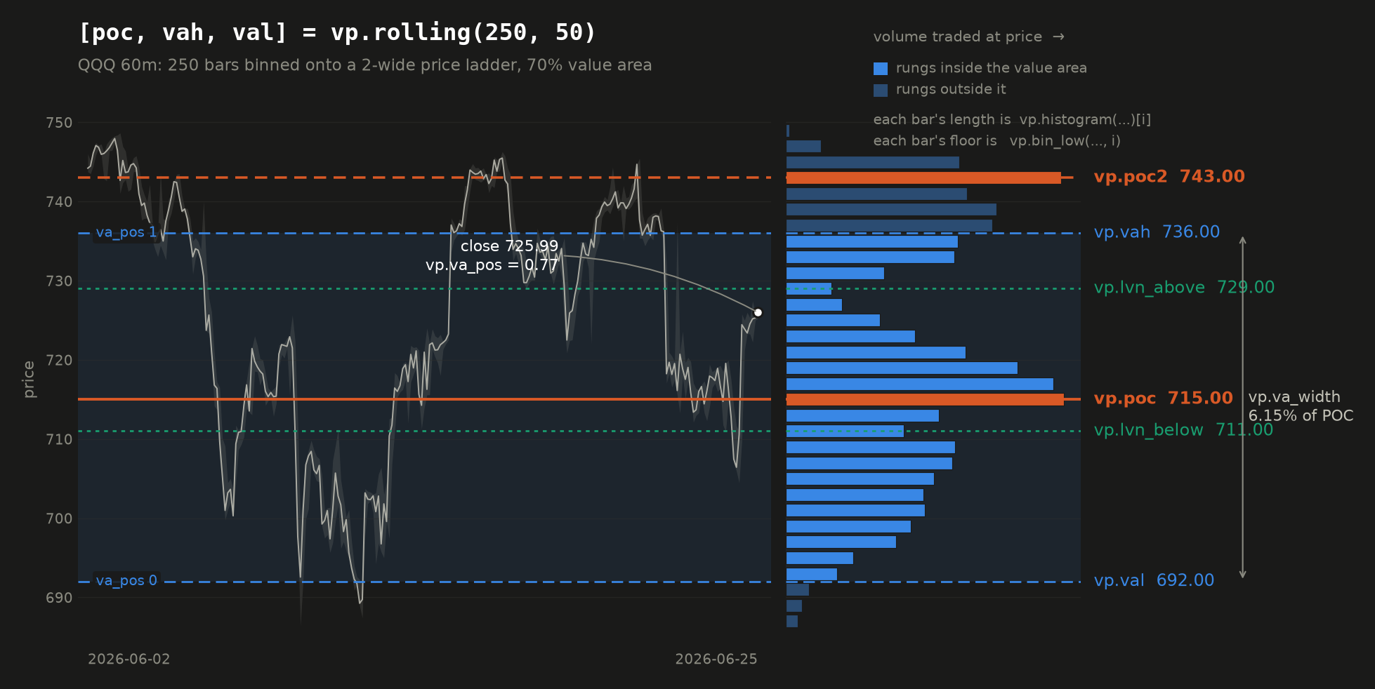
Every reading the namespace offers is on that figure, and every number on it is the one vp.*
returns for that window. The histogram on the right is the profile itself, one bar per rung of the
price ladder; the levels drawn across both panels are what the calls below hand back. This
particular window is bimodal, which is why it is the one drawn: the market traded around two
prices rather than one, so there is a vp.poc2 to show as well as a vp.poc.
Reading it in Pine
//@runtime=2026.08.14-vp
//@version=6
strategy("Value area gate", overlay = true)

[poc, vah, val] = vp.rolling(500, 50)

// take an existing signal only at a discount to the volume-agreed price
raw = ta.crossover(close, ta.sma(close, 20))
if raw and not na(poc) and close < poc and close > val
    strategy.entry("L", strategy.long)

if strategy.position_size > 0 and close > vah
    strategy.close("L")
There are three ways to choose which bars go into the profile:
| call | the bars it profiles |
|---|---|
vp.rolling(length, bins, va) | the last length chart bars |
vp.session(anchor, bins, va, id) | everything since anchor was last true |
vp.intrabar(tf, length, bins, va) | the same rolling window, binned from a lower timeframe |
All three return [poc, vah, val]. Then the readings off a rolling profile:
| call | returns |
|---|---|
vp.poc(length, bins) | the point of control on its own |
vp.poc2(length, bins, sep) | the second point of control, or na when the profile has only one mode |
vp.vah(length, bins, va) / vp.val(length, bins, va) | the value area edges on their own |
vp.va_pos(length, bins, va) | where the close sits inside the value area: 0 at the low edge, 1 at the high |
vp.va_width(length, bins, va) | the value area's width as a percent of the POC |
vp.lvn_below(length, bins) / vp.lvn_above(length, bins) | the nearest low-volume node below or above price |
vp.histogram(length, bins) | array<float> of bin volumes, lowest price first |
vp.bin_low(length, bins, i) | the price floor of bin i of that histogram |
bins defaults to 50 and va to 0.7. The single-value calls are not a slower path: all of them
share one cached window per set of arguments and one result per bar, so reading all three levels
costs the same as reading one.
The session profile
vp.session accumulates instead of sliding. You give it a bool that says "start again", and it
profiles everything since that last fired. A daily profile is the usual case:
newDay = ta.change(time("D")) != 0
[poc, vah, val] = vp.session(newDay, 50)
Two differences from vp.rolling are worth knowing. It answers from the first bar of a
session rather than waiting for a window to fill, so early-session levels are thin and built from
very few bars. And it must be called on every bar: the anchor is something your script decides
per bar, so a bar the call was skipped on has no anchor that could be recovered.
The id (default 0) exists only if you run more than one session profile. The identity of a
session is its anchor, and an anchor is a bool arriving each bar rather than something the call can
be recognised by, so two profiles with different anchors need different ids or they would share one
accumulation and both be wrong.
Low-volume nodes
A node is the opposite of the POC: a thin band price moved through rather than traded at, which is where it tends to move quickly again. That makes it a natural place to put a stop, past the void rather than at a round number.
stop = vp.lvn_below(500, 50)
if not na(stop)
    strategy.exit("X", "L", stop = stop * 0.999)
It finds a dip the profile comes back up from, rather than simply the thinnest bin. A profile
always thins out toward its edges, so "thinnest" would nearly always answer with the outermost bin:
true, and useless. Where there is no gap on that side of price, the call returns na, which is an
ordinary outcome to guard rather than an error.
The second point of control
A market does not always agree on one price. It can spend a window trading around two, moving
quickly between them, and a profile of that shape has two humps rather than one. vp.poc is a
single argmax, so it names the larger and says nothing about the other. vp.poc2 names the other.
poc = vp.poc(500, 50)
second = vp.poc2(500, 50)
if not na(second)
    // the market has two acceptance zones, and the void between them is the node
    mid = vp.lvn_below(500, 50)
It is not "the next-heaviest rung", and that distinction is the whole feature. The rung beside the point of control is heavy for exactly the reason the point of control is, so any second-highest reading answers with the POC's own neighbour: a number that is always available, always plausible, and never means anything. A second peak is a second mode only if the profile comes back down between the two.
sep is that test, and it is a ratio rather than a volume so it does not move with the instrument
or the window length. It says two things at once, which at the default both read as "half":
- the valley between the peaks must give back at least
1 - sepof the smaller hump, and - that hump must be worth at least
sepof the larger one.
The second half is what keeps the answer out of the profile's own tail, where a one-rung wiggle
clears any valley test trivially because everything around it is near zero. Lower sep to demand
a deeper, more convincing void; raise it to accept a softer separation. na is the ordinary
answer on a single-mode profile, not an error, and a strategy guards it exactly as it guards
vp.lvn_below.
Profiling the lower timeframe
Binning a chart bar spreads its volume across the whole range that bar covered, which is a guess:
the bar does not record where inside its range the trading happened. vp.intrabar uses a finer
series instead, so the volume lands where it actually traded.
[poc, vah, val] = vp.intrabar("5", 500, 50)
The window still slides one chart bar at a time; only the resolution inside each bar changes.
It needs the job to have a lower-timeframe series (the same one request.security_lower_tf reads),
and it says so plainly if there isn't one rather than returning na, which would be
indistinguishable from warmup.
What to know before you build on it
- It returns
nauntil the window is full. Guard withnot na(poc). A rolling profile is not defined on a partial window, so there is no partial answer to give you. - An instrument with no volume is refused, loudly. Cash indices carry no traded size on any
data source, and Saxo's FX and CFD bars have no volume field at all. Rather than hand back a
"point of control" that is really just the midpoint of the window,
vp.*stops the job and names the symbol. Do not put it on DAX 40, CAC 40 or an FX pair. - Sweep the window freely. The profile slides (one bar in, one bar out) instead of being
rebuilt, so its cost does not grow with
length. Measured over 5,000 bars, a 2,000-bar window costs the same per bar as a 100-bar one, and less thanta.highestover the same window. - It is built from bars, not ticks. Each bar's volume is spread across the price range that bar covered. That locates where trade concentrated; it is not an exchange volume-at-price feed.
- It needs no extra data. Unlike
gex.*, which needs a live options chain, a volume profile is computed from bars the job already has. So it behaves identically in a backtest, a sweep and a live bot, on every broker. - Pin the runtime.
vp.*needs//@runtime=2026.08.14-vpor later, andvp.poc2needs//@runtime=2026.08.23-poc2or later.
As a machine-learning feature
The same reading is available to the model trainers as Distance from
volume POC (vp_dist_poc): the percent distance from the close to the point of control, over a
lookback you choose.
It is a distance, never a price. A model trained on an absolute level learns a threshold that sits on one side of every later price range, so the feature quietly goes dead as soon as the market leaves the range it was fitted in. Everything in that catalogue is relative for this reason.
It also needs an instrument that reports volume, and the fit refuses one that does not rather than training on a column of zeros.
Live Trading
Deploy a strategy as a live bot that connects to a broker and executes orders in real time.
Available on every plan. The Free plan includes 1 live trading job with a limited lifetime (bots are stopped at the end of the trading day); Pro and Premium raise the concurrency limit and run without that daily stop.
Live trading is open to everyone; three options on the launch form are not. Basket and Portfolio mode and the Webhook URL need Pro, and a strategy that reads a second timeframe needs Premium. Each is marked on the form, and the refusal names the plan rather than failing at the broker.
Launching a bot
- Go to Live and connect a broker (see Brokers).
- Select a strategy and symbol, or tick Basket to trade several symbols with one bot (see Multi-symbol baskets).
- Choose the timeframe (
5m,15m,30m,60m,90m,1D; see Timeframe syntax). - Enable Auto-restart if you want the bot to restart automatically after a crash.
- Check the Execution routing card below the form. It decides where the orders actually go (see Execution routing).
- Click Launch.
Monitoring
Running bots are listed with their status (running, stopped, failed). Click Logs on any bot to stream its container output in real time. Bot lifecycle events (started, stopped, crashed, restarted) are recorded in the event log and can be exported as CSV.
Next to the status is the exchange's own session phase, because a quiet bot is ambiguous until you know whether its market is trading: at 20:00 CET a US equity bot with no new bars is stalled, an EU one is asleep until the morning. The phase comes from the broker's calendar, never from a market-hours table of ours, so a holiday, a half-day or an opening auction reads as what it is rather than as a fault in the bot. Green is continuous trading, red is shut, amber is everything in between (an auction, extended hours, the daily break) or an unreachable venue. Hover for the source.
| Broker | Where the phase comes from |
|---|---|
| Alpaca | The account's market clock, with the next open and close. |
| Saxo | The instrument's exchange and its session windows, in the exchange's own words: automated trading, opening auction, pre market, trading at last, closed. |
| Prop futures (Tradovate) | The product's regular Globex schedule as Tradovate publishes it, in Chicago time: automated trading through the week, daily break in the 16:00 to 17:00 maintenance hour, closed from Friday 16:00 to Sunday 17:00. Holidays are not covered: the venue's schedule endpoint carries none, so a CME holiday reads as open. Read once a day per product, because every Tradovate login counts against the account's two-session cap and the oldest session evicted would be your bot's. |
| Bitstamp | Crypto never closes, so always continuous. |
| Binance, Interactive Brokers, Lightspeed | No session source is wired for these yet, so the column reads unknown. It is never guessed: saying closed would invent a fault. |
If Telegram notifications are configured, each bot also sends a periodic heartbeat. A multi-symbol basket sends a single combined overview: one message with a per-symbol table (price, position, live P&L) and a net-P&L summary, colored green/red by profit and loss:
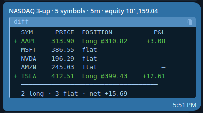
Auto-restart
When auto-restart is on, the platform will restart the bot automatically if it crashes, up to a configured limit. The restart count is shown on the bot card.
Fleet snapshot
Auto-restart handles one bot crashing. It does not help when the machine underneath them goes away.
A live bot is a container on a runner host. The platform's own services can restart without disturbing a running bot, but if the runner host reboots or its Docker daemon restarts, every container stops at once. Nothing is lost (positions are at your broker, and each bot's trade log survives on disk), but you come back to an empty Active bots table and, without a snapshot, you relaunch each bot by hand.
Save snapshot records which bots are running. Restore fleet starts them all again in one click.
You keep one snapshot: the last one you saved. Saving again replaces it, which is how you record a fleet you have changed. Stop the bots you no longer want, then save again. To discard a snapshot entirely, stop everything and save with nothing running.
Both buttons sit next to Start Bot on the Live Bot Manager, because they are the same job at two scales: Start Bot launches one, Restore fleet launches the set.
Restore is never automatic, and that is deliberate. After a real outage your broker credentials are usually gone too. A Saxo refresh chain expires within the hour, and logging out clears stored broker tokens by design. An automatic restore would fire a row of doomed launches at dead credentials before you had a chance to reconnect. So:
- Reconnect your broker.
- Press Restore fleet and confirm. The dialog names the bots that will start.
A partial restore is normal, and the result names every bot that did not start along with the reason: a broker not yet reconnected, a runner still offline, or your plan's concurrent-job limit reached. Bots already running are left alone, so pressing Restore twice is safe.
Restoring reuses the original bots rather than creating copies, so each one keeps its trade history and picks its position back up at the broker exactly as a crash-restart would. If you launch new bots after saving, the page tells you the snapshot no longer matches what is running, so you can save again. It is never updated silently.
Performance
Live → Performance compares your running bots against each other. It is realized only: a trade enters the figures when it closes at a price the broker gave us, and not before. Open positions have no result yet and live on their own page.
Every figure is a ratio, never an absolute amount, because absolute figures are not comparable
between bots. A round trip is scored as (exit − entry) / entry, a price return, so a €500
account and a €500,000 account running the same strategy on the same instrument produce the same
number, and bots on different brokers, currencies and timeframes can be ranked side by side.
| Column | What it tells you |
|---|---|
| Avg / trade, Median | The edge per trade. A large gap between them means one outlier is carrying the average, which is common at small sample sizes. |
| Sharpe | Reward per unit of risk (mean ÷ standard deviation of the trade returns). The closest single number to "better". |
| SQN | The same ratio scaled by how much evidence backs it, so a bot with two lucky trades cannot top the ranking. The table sorts on this by default. |
| Exposure, % / mkt-day | How hard the capital worked rather than sat idle. Two bots at the same return per trade are not equivalent if one is in the market 10% of the time and the other 90%. |
| Share | What fraction of the position size deployed on that account this bot is getting. |
| Max DD, Max L | Worst fall of the cumulative trade-return series, and the longest losing run. |
Every column sorts (click again to reverse) and every column filters: contains on the text
columns, min/max on the numbers. A row near the top on SQN and near the bottom on Share is a
strategy earning well on less of the money than its peers. The page shows that and stops there;
it does not tell you what to do about it.
Two things these numbers are not. They are gross: commissions and broker fees are not included, so they are not comparable with your backtests, which run a 0.2% commission; a strategy with a real but sub-fee edge looks fine here and is not. And they are strategy performance, not account performance: every figure comes from what the bot itself did, so trades you placed by hand in the same account, fills that landed after a bot stopped, and broker liquidations are not in them. Your broker account remains the source of truth for money.
Sharpe is deliberately not annualised: scaling it by trades-per-year needs a rate a two-day-old bot does not have and assumes trades are independent, which they are not. Read it as reward per unit of risk, per trade.
A position that vanishes at the broker is recorded, not forgotten. A resting stop that filled between two polls, a close you made by hand, a margin liquidation: the bot notices at its next sync and books the round trip as closed on every broker, so the Open positions page stops showing a position your account no longer holds. That stale belief is the dangerous one, because it is what makes someone reach for a manual close, and a sell with nothing behind it is a short. Where the venue gives us no price for that exit (the crypto exchanges reconstruct a cost basis from your fill history and have no exit equivalent), the trade is booked without one and lands in unscored exits: it is reported as having happened, and it is left out of the P&L figures rather than scored from a guess. Dropping those instead would bias the record, because a liquidation is not a randomly distributed outcome.
Bars under about ten closed trades are flagged: a ranking built on two trades is luck, not edge,
and the Trades column's min filter is the first one to reach for.
How orders are executed
It is important to understand how a live bot turns a strategy signal into a broker order:
- Bots act on bar close. On each new completed bar, the bot evaluates your strategy. A plain
strategy.entrybecomes a market order at that moment. limit=andstop=become real broker orders.strategy.entry(limit=…)places an actual resting limit order at your broker; it may fill later, or never. Andstrategy.exit(limit=…, stop=…)places a native OCO pair on Saxo and Alpaca equities: a resting stop and a resting take-profit, linked by the broker so that whichever one fills cancels the other. The stop moves as your strategy trails it.- The entry price is the broker's real fill, not the bar close. The bot reads the executed price back from the broker (Saxo, Alpaca, Bitstamp), so
strategy.position_avg_price, and any stop or target computed from it, is based on what you actually paid, not on a bar close that is already minutes stale. - Every order carries a reference back to the bot that placed it. Orders are tagged
pcx-<strategy>-<job>-…in your broker's own order history (Alpaca and Bitstampclient_order_id, SaxoExternalReference), so a trade in your broker's report can be traced to a specific bot rather than guessed at from the symbol and the time, which is ambiguous as soon as two bots on one account trade the same instrument. - PineconeX does not track your live profit & loss. It records lifecycle events (started, stopped, crashed) and the signals it acted on, but it does not reconcile partial fills or rejections into a running P&L. Your broker account is the source of truth for real positions, fills, and P&L, so always confirm there.
Live results can still differ from a backtest on identical signals: a backtest fills at modelled prices at the bar close, while a live order fills at whatever the market gives you, and a live resting stop can be hit inside a bar, where a backtest would only have seen the bar's close. The divergence is by design: live is native, backtest is simulated.
Stopping a live bot cancels its resting orders; it does not close the position. On shutdown the bot cancels the entry and exit orders it left at the broker (a resting order with no bot behind it is a hazard: a stop-loss is a sell, and a sell with nothing behind it can open a short). What it holds is yours, so it is left alone and named in the log as unprotected. Close the position yourself in your broker's interface if you do not intend to relaunch, since a relaunched bot re-adopts the position and re-protects it. (On Bitstamp nothing rests at the exchange in the first place, see Crypto.)
Order flow: what each broker supports
Your Pine Script is identical on every broker. What the broker does with the order is not, and the differences are not cosmetic: on one venue a stop-loss rests at the exchange and fires while you sleep, on another there is no stop order at all and the bot has to do it.
The PineconeX column is what the platform sends, and how you ask for it in Pine. The venue columns are what happens to it once it arrives. A gap in the first column is ours; a gap in a venue column is the venue's, and no amount of platform work will close it.
| PineconeX | Saxo (stocks, futures) | Alpaca equities | Alpaca crypto | Bitstamp spot | Binance spot | Prop futures (Tradovate) | |
|---|---|---|---|---|---|---|---|
| Market entry and close | strategy.entry / strategy.close | Yes | Yes | Yes | Yes | Yes | Yes |
| Limit entry | strategy.entry(limit=) | Yes | Yes | Yes | Yes | Yes | Yes |
| Stop entry | strategy.entry(stop=) | Yes (StopIfTraded) | Yes | Sent as stop-limit | No | Sent as stop-limit | Yes |
| Resting stop-loss | strategy.exit(stop=) | Yes | Yes | Yes (the one resting slot) | No | Yes (the one resting slot) | Yes (bracket) |
| Resting take-profit | strategy.exit(limit=) | Yes | Yes | Bot-managed | Bot-managed | Bot-managed | Yes (bracket) |
| Stop and target linked by the venue | Sent as one OCO where it exists | Yes | Yes | No | No | No | Yes (bracket on the entry) |
| Trailing a stop | Re-sent whenever your script moves the level | Amended in place | Cancel and replace | Bot-managed | Bot-managed | Cancel and replace | Cancel and replace |
| Cancel a resting order from your script | strategy.cancel / strategy.cancel_all, resting entries only | Yes | Yes | Yes | Yes | Yes | Yes |
| Shorting | strategy.entry(direction=strategy.short) | No on stocks, yes on futures | Yes, if your account allows it | No | No | No | Yes |
| Order quantity | Sized by your strategy, rounded to the venue's unit | Whole units | Whole units | Fractional | Fractional | Fractional, on the venue's step | Whole contracts |
"Bot-managed" means the level is real but it lives in the bot, not at the venue: it is checked at each bar close, and when it is hit the bot cancels whatever else is resting and closes at market. That is a genuine protection, but it cannot fire between two bars. If price gaps through the level overnight or over a weekend, you exit on the next bar close at whatever the market is then.
PineconeX does not use a venue's own trailing-stop order type even where one exists. Your script owns the level: it recomputes the stop each bar and the bot moves the resting order to match, so a trail written in Pine behaves the same on every broker and matches what your backtest did. A native trailing order would follow the venue's rule instead of your script's.
Where a venue simply does not have the order
- Bitstamp spot has no stop order, no take-profit and no OCO. It is an exchange order book with
market and limit orders, and nothing else. Worse, its API accepts a stop price and answers
200 OKwith an order id while creating nothing, so a bot that trusted the response would report a stop that does not exist. PineconeX never claims one: every Bitstamp stop and target is bot-managed, on a market that trades 24/7. See Crypto. - Alpaca crypto allows one resting exit per position. The first resting order reserves the whole coin balance, so a second leg is refused. That slot is given to the stop, because it is the protection, and the take-profit is bot-managed.
- Binance spot allows one resting exit per position, for the same reason: a resting sell
reserves the base balance. The stop takes the slot and the take-profit is bot-managed. Unlike
Bitstamp, the stop it rests is real, so a Binance bot is protected between bars. A pair whose own
orderTypesdo not listSTOP_LOSS_LIMITis demoted to the bot-managed stop, and the bot says so at startup rather than assuming. - Bitstamp and Binance are long-only. A short entry is refused before it reaches the exchange: there is nothing to borrow on spot.
- Saxo stock accounts do not short. A sell with no holding behind it comes back
NotOwned, even on a margin-enabled account. Saxo futures do short. - Alpaca options take limit, stop and stop-limit, but no OCO, bracket or trailing order. Options routing is described under Options routing (Alpaca).
Rules that catch people out
- A resting exit only exists while the position does. Saxo refuses an exit order placed against nothing, and every venue has its exits cancelled before the bot closes at market. Cancel first, then close, is the order everywhere, and it is why stopping a bot cancels its orders rather than leaving them behind.
- Saxo polices where an exit may sit. A take-profit on the wrong side of the market, or too far from it, is rejected. Because an OCO is a single request, a rejected take-profit used to take the stop down with it, so PineconeX now retries the stop on its own: a position with a stop and no target is managed, the reverse is not.
- Saxo prices snap to the instrument's tick grid, which is banded by price level (finer on a cheap instrument than an expensive one). Your level is rounded to the nearest valid tick before it is sent, so the resting order can sit a tick away from the number in your script.
- A rejection can arrive as
200 OK. Bitstamp and Tradovate both report refusals inside a success response. PineconeX reads the body rather than the status code and surfaces the venue's own error in your job log. strategy.cancelwithdraws a resting entry, and cannot touch a protective exit. A cancel naming an entry that is resting at the broker takes it off the book, andstrategy.cancel_alltakes off whatever is resting. Your stop and take-profit are deliberately out of reach: they are what stands between an open position and an unbounded loss, so they come off when the position does (a close cancels its exits first, in that order) rather than on a script's say-so. A cancel that matches nothing does nothing and says nothing, because calling cancel on every bar is ordinary Pine. New in v0.2.0-alpha: try it on paper or a simulation account before you rely on it live.- Time in force is per venue. Alpaca equity orders are day orders and die at the close; Alpaca crypto and every futures bracket leg are good-til-cancelled.
Execution routing
The Execution routing card on the launch form decides where a signal ends up. There are three routes, and they combine:
| Route | What it does |
|---|---|
| Execute orders on the broker | The default. PineconeX places the order on your connected broker account. Unchecking it makes the bot signal-only: it evaluates the strategy, fires the webhook, and sends nothing to your broker. |
| Webhook URL | Order events are POSTed to your own http(s) endpoint: the strategy's alert_message when it has one, a structured event otherwise. Mainly to hand execution to a third-party platform, but usable for plain notifications. Delivery only ever goes to the address you enter. |
| Options routing | Alpaca only. Each signal is scored across the shares and the option chain, and the better expression is placed. See below. |
If a third-party platform executes off your webhook, it owns the real position. PineconeX then only tracks its own simulated one, which can drift from your actual account.
Delaying order submission (runtime.sleep)
A bot submits its orders the moment it notices a bar has closed. That is fine for one account, but it has a side effect worth knowing about: for a given bot, the gap between the bar close and the order is very nearly the same on every single bar. The orders land on a metronome.
runtime.sleep(ms) breaks that up. Call it in your strategy and the bot holds the orders that bar
produced for the number of milliseconds you ask for, then submits them:
//@version=6
strategy("Delayed submission", overlay = true)

// A different, repeatable delay on every bar, anywhere from 30 to 240 seconds.
seed  = input.int(7, "Delay seed")
h     = math.sin(bar_index * 12.9898 + seed * 78.233) * 43758.5453
u     = h - math.floor(h)
delay = 30000 + u * 210000
runtime.sleep(delay)

if ta.crossover(close, ta.sma(close, 20))
    strategy.entry("L", strategy.long)
Not to be confused with
runtime.exit, which ends a run instead of delaying an order, and works in every run type rather than only in a live bot.
It only ever affects a live bot. A backtest, a sweep, a significance run and a stress run all read the request and ignore it, because a bar-resolution simulation has no prices between one bar close and the next, so there is nothing to fill at a sub-bar offset. The backtest says so once in its log rather than passing over it silently, since unchanged fills could otherwise be read as evidence that a delay costs nothing. Adding it to a strategy cannot change a single number in any result you have already recorded.
Four things to know before you use it:
- It is capped at the length of one bar. A delay that outran the bar would submit an order for a decision the next bar has already replaced, and the next bar posts its own request, so the two would overlap. On a 5 minute chart anything above 300000 ms is cut to 300000.
- It is refused outright on a
calc_on_every_tickstrategy, with a warning in the job log. A tick strategy exists to act the instant its signal becomes true, so holding its order back asks for the opposite of what it declared. See Tick data vs. bar data. - It never delays an exit. Stops, targets, the risk halt and the end of session flatten are all handled before the delay is applied, so getting out of a position is never postponed.
- Give every account its own seed. Two bots on the same seed draw the same delay for the same bar, which puts their orders back in lockstep and recreates exactly the pattern the delay is there to remove.
Note that your bot already submits somewhat after the bar close without asking: it polls for new
bars on a timer, so it notices a completed bar up to half a bar late. runtime.sleep adds to that
offset rather than replacing it, and what it really changes is that the offset stops being
constant.
Options routing (Alpaca)
Tick Let the model choose shares, calls or puts per signal and each signal is scored by a pricing model across the underlying shares and the option chain (a long can be expressed by buying shares or calls, a short by buying puts), and whichever gives the better risk-adjusted outcome is placed. A long option's premium is a hard maximum loss; a stop is not, because a gap can trade straight through it.
It is a fit question, not a feature toggle. Options routing suits fast, directional strategies: momentum, breakouts, catalysts. On a slow or mean-reverting strategy the option decays while it waits for an exit signal and can expire worthless, losing the premium where the shares would have sat roughly flat. If the edge is not a near-term move, use shares.
Each bot carries its own settings; leave a field blank to use the runtime default shown as the placeholder:
| Setting | Meaning |
|---|---|
| Capital ($) | Cash the model may deploy per signal. |
| Risk fraction (0–1) | Fraction of that capital allowed to be lost on the stop; this is what sizes the position. |
| Horizon (days) | How long you expect to hold. Drives which expiry wins the scoring. |
| Min DTE / Max DTE | The expiry window the chain search considers, in days to expiry. Min DTE is floored at 1, so same-day (0DTE) contracts are unreachable from the product. |
| Auto-roll before expiry | On by default. A held option is rolled to a later expiry before it decays to nothing: the chain is re-scored exactly as the entry was, the near leg is closed and the further one opened. Your strategy reasons in the underlying's price and is blind to expiry, so without this a sideways market with no exit signal can let a position expire out from under it. |
| Allow short | Open a short expression when a sell signal arrives with nothing held. |
| Dry run | Score and log the decision, place nothing. The safe way to watch the model on a live feed. |
Multi-symbol baskets
Pro plan and above, as is Portfolio mode, and the portfolio backtest and sweep that share the same book model. Tick Basket on the launch form to have a single bot trade several symbols in one process, over one shared timeframe and one broker account, instead of launching one bot per symbol. It counts as one job against your concurrency limit.
- One combined heartbeat. A basket sends a single Telegram overview, a per-symbol table (price, position, live P&L) plus a net summary, rather than one message per symbol.
- One position per symbol, evaluated at the same bar close across the basket.
- Saxo, Alpaca, Bitstamp and Binance only. Interactive Brokers and Lightspeed do not fit a shared connection, and a prop-firm futures basket would be a basket of contract months with its own roll for each, so single symbol only there.
Launching one bot per symbol remains the more controllable option: each has its own log, its own position and its own stop button, so you can shut one symbol down without touching the rest.
Margin monitoring
A live bot checks the account's margin usage every 5 minutes on every broker that can lend (Saxo, Alpaca and prop-firm futures) and reports it in the log, so a margin call is visible before it acts on you. Bitstamp and Binance spot cannot borrow at all, so no margin call is possible there.
Margin is consumed by borrowing, not by holding: a cash-funded long uses none, and a bot on such an account simply logs "no leverage in use". A blocked or restricted account is reported as such rather than as a healthy 0%. Note this is your broker's limit; the strategy's own cap is margin_long / margin_short, and the two are enforced independently.
Crypto
Crypto trades on Bitstamp (USD and EUR spot pairs), Alpaca (US-dollar pairs) and Binance (USDT pairs). Pick the symbol under the Crypto (USD) or Crypto (EUR) index; the symbol list shows which venues carry it.
Your Pine Script does not change. What the broker does underneath changes a great deal, and the single most important difference is what actually protects your position:
| Venue | Stop-loss | Take-profit |
|---|---|---|
| Saxo / Alpaca equities | Native, resting at the broker | Native, resting at the broker (OCO: a fill on one cancels the other) |
| Alpaca crypto | Native, resting at the broker | Managed by the bot: crypto allows only one resting exit, and that slot is given to the stop. The bot checks the target at each bar close and, when hit, cancels the stop and closes at market. |
| Binance spot | Native STOP_LOSS_LIMIT, resting at the exchange | Managed by the bot: one resting exit only, same as Alpaca crypto and for the same reason. |
| Bitstamp | Managed by the bot: Bitstamp spot has no stop order at all | Managed by the bot |
A Bitstamp stop-loss is not held at the exchange. Bitstamp's spot market has no stop orders, no take-profits and no OCO, and the API even accepts a stop price and answers
200 OKwith an order id, while creating nothing. So PineconeX never claims one: on Bitstamp, your stop is enforced by the bot, at bar close. If price gaps straight through your stop level between two bars, the bot exits on the next bar close, at whatever the market is then, not at your stop price. On a 24/7 market that gap is a real risk. Size accordingly, and prefer a shorter timeframe if the stop matters to you.
Other crypto specifics worth knowing:
- Crypto never closes. There is no session, no end-of-day. A bot on a 5m crypto chart runs through the night and the weekend.
- Size is fractional. Unlike equities, crypto orders are not rounded down to whole units:
0.0134BTC is a valid order. Binance rounds to the pair's ownstepSizeand refuses anything under its minimum notional, rather than rounding it for you; the bot reads both at startup and prints them. - Fees land in different places. On Alpaca and Binance the fee is taken in the coin (order 0.001 BTC, own slightly less); on Bitstamp it is taken in the cash (order 0.0002 BTC, receive exactly 0.0002 BTC). The bot sizes its exits from what the broker says you actually hold, so this does not strand dust, but it explains why the filled quantity may not equal the ordered one on Alpaca and Binance.
- None of the three venues allows shorting crypto. A short entry is refused.
- A Binance pair is quoted in USDT, and the rest of the symbol is quoted in USD.
BTCUSDcarries a Yahoo, a Bitstamp and often an Alpaca id in real dollars, and its Binance leg isBTCUSDT. The two track within a few basis points normally and they do not during a stablecoin depeg, which is exactly when a crypto strategy is busiest. A backtest on that symbol runs on USD bars while a Binance bot fills in USDT. Position sizing is unaffected: the bot sizes against the account's real USDT balance.
Tick data vs. bar data
Everything else in PineconeX works on bars. A bar is the smallest unit of time the engine knows about: your strategy runs once, at the close of each completed bar, and sees the five OHLCV numbers that summarise it (see What a bar contains). Everything that happened inside that bar, the individual trades, the bid/ask spread, whether the high came before the low, is gone by the time your script runs.
Tick data is the layer underneath. A tick is a single event on the wire: one trade printed, or one change at the top of the order book. On a liquid US stock that is roughly 45 events per second, peaking above 240: thousands of ticks compressed into the four prices of a single 5-minute bar.
PineconeX can run a strategy on that layer instead, in a live bot only, through two pieces that work together:
| What it does | |
|---|---|
calc_on_every_tick=true | Re-runs your whole script on every real-time tick, against the still-forming bar, instead of once at bar close. |
tape.* | A namespace giving the script read access to the tick itself: the last trade price and the top-of-book quote. |
This goes beyond TradingView, and is not portable. TradingView's
calc_on_every_tickre-runs a script per tick but exposes no tick-level data, so the script still only sees the forming bar's OHLC.tape.*is a PineconeX-exclusive namespace, likeml.*andgex.*. A script using it will not run on TradingView.
Preview feature. The tick engine ships only on runtimes that include it, so pin one with a
//@runtime=line at the top of the strategy, as GEX does, or ask support which default runtime carries it. Today the tick path is observation-first:tape.*and the signals it produces are evaluated and logged on every tick, while order placement stays on the bar-close path unless intrabar ordering is enabled for your bot (see What actually gets ordered).
Enabling it
There is nothing to switch on in the interface. It is declared in the strategy itself, as an
argument to strategy():
//@version=6
strategy("order flow", overlay=true, calc_on_every_tick=true)
That is the whole switch. When a bot launches, it checks each strategy in its basket for the flag, and attaches a real-time feed only if at least one asks for it. A strategy without the flag behaves exactly as before: one evaluation per completed bar.
Backtests, sweeps and validation ignore it completely. There is no tick history to replay: the
catalog stores bars, not ticks. In a backtest, a sweep, a significance or stress run, and in the
inline validator, every tape.* field reads na, so a tick strategy shows no trades at all.
This is deliberate and safe (a missing tick can never produce a garbage price level), but it means
a tape.* strategy cannot be backtested. You cannot validate its edge the normal way; treat
anything you build here as unproven until you have watched it on a paper account.
Which feeds carry ticks
Tick data comes from a broker's streaming socket, not from the data catalog, so it depends entirely on the data source your bot is running:
| Source | Tick feed | Notes |
|---|---|---|
| Alpaca (US equities) | Yes, real-time | The free IEX tape by default (a few percent of consolidated volume). The paid consolidated SIP tape is an operator setting. |
| Alpaca (crypto) | Yes, real-time | 24/7, so a tick strategy can be observed outside market hours. |
| Bitstamp (crypto) | Yes, real-time | Public feed, no API key needed: live trades and the top of the order book, 24/7. |
| Saxo Bank | Yes, but delayed | Quote-only and typically ~20 minutes behind without a real-time market-data subscription. Observe-only, see below. |
| Binance (crypto) | No | No tick path yet. calc_on_every_tick is accepted, warns in the log, and the strategy runs once per bar close. |
| Prop futures (Tradovate) | Yes, in preview | Real trade prints and quotes on the front-month contract. Untested against a live prop-firm account, so treat tape.* there as unproven. The feed reports no entitlement of its own, so the bot measures its own delay and will not place an intrabar order on a feed it cannot show is real-time. |
| Yahoo, Massive, Interactive Brokers | No | No tick path. calc_on_every_tick is accepted and simply never fires. |
If a strategy asks for ticks on a source that has none, the bot says so in its log and carries on at bar close; it does not fail to start.
Alpaca allows one market-data connection per account, and PineconeX now shares it. Your tick-streaming bots on one Alpaca account read a single upstream connection between them, so several can stream at once where previously the second was refused. The connection is opened only when a bot actually needs it and released about a minute after the last one stops, so a bot that does not set
calc_on_every_ticknever takes it. Equities and crypto are separate feeds, so one account can hold both. The sharing is per server: bots for one account are placed on the same server where there is room for them, and a bot that has to be placed elsewhere is refused the stream and falls back to bar close. It still trades normally either way, since orders and bar polling go over REST and onlytape.*is affected.
The tape.* namespace
Every field is a series float, and every one is na until a tick supplies it:
| Field | Meaning |
|---|---|
tape.price | Price of the last trade on this tick. |
tape.bid / tape.ask | Top-of-book quote: the best bid and best offer. |
tape.bid_size / tape.ask_size | Size resting at the top of the book (order-book imbalance). |
na is the safe default everywhere: in a backtest, before the first tick arrives, during warmup,
and on a partial tick. Many feeds send trades and quotes as separate events, so a trade-only tick
leaves tape.bid/tape.ask at na and a quote-only tick leaves tape.price at na. Guard
every read, not na(tape.price), exactly as the smoke strategy below does. Non-finite values
are filtered out of orders and stops downstream, so an unguarded strategy does nothing rather than
firing at a nonsense price, but the guard is what makes the logic explicit.
There is no tick lookback. tape.price[1] reads na: the engine keeps no per-tick history, so
each re-run sees only the current tick plus the committed bar history. Anything comparing this tick
to the last one has to derive it from bar state.
Saxo's tape is not a trade tape. A Saxo price subscription streams Bid/Ask/Mid, with no trade prints, so
tape.priceis the mid, which by construction always sits inside the book. Any signal of the form "the trade lifted the offer" (price >= ask) is unsatisfiable on Saxo. The streamed quote also omits size, sotape.bid_size/tape.ask_sizeare unusable there. Combined with the delay, Saxo's tick path is for observation only; never let a stale quote drive an order.
How often your script actually re-runs
Not on every tick. A liquid symbol can push hundreds of events per second, and re-running a whole strategy that often would simply fall behind. Instead the bot coalesces: every arriving tick is merged into a per-symbol accumulator (cheap, since it just overwrites the latest trade and quote), and the script re-runs once on the freshest merged state, no more often than that symbol's own cadence.
That cadence is derived from your strategy, not configured. At warmup the bot times 200 real re-runs of your script and spaces re-runs at 4× the measured cost, clamped between 5 ms and 1 s. A cheap strategy therefore re-runs at close to tick speed; a deep-history one spreads out. The bot prints the measured figure when it starts:
[AAPL] intrabar re-run ≈310µs → coalesce ≥5ms between re-runs (≤200/s), 4× margin
Two consequences worth internalising:
tape.*is the latest tick, not every tick. Trades that arrived between two re-runs were merged, not queued. You cannot count prints, sum tick volume, or reconstruct a trade sequence from it: it is a live snapshot of the tape, not a recording of it.- A heavier strategy sees a coarser tape. If you need reaction speed, keep the tick path's logic short and let the expensive indicators run at bar close.
Writing tick logic: the one rule that surprises people
Each intrabar re-run happens on a throwaway clone of your script's state. The committed state only ever advances at a real bar close. That is what makes it safe to re-run the same forming bar hundreds of times, but it also means:
Anything written to a
varduring a tick re-run is discarded. Avarcounter incremented on every tick will appear to advance only once per bar, because only the bar-close run is kept.
So tick logic must be stateless: derivable from the current tape.* values plus committed bar
state. If you need memory across ticks, it belongs in the bar-close path.
Deduplication works the normal Pine way. A signal that is true intrabar will still be true on the next re-run a few milliseconds later, so guard entries with the position itself:
if liftOffer and strategy.position_size == 0
    strategy.entry("L", strategy.long)
When a fill happens, the bot reflects it back into the committed state immediately, so the very next re-run sees the position and the entry cannot fire twice.
What actually gets ordered
The tick path is being rolled out in stages, and the current default is conservative:
- Observation (default). The script re-runs per tick,
tape.*is live, and the orders the strategy would emit are counted and logged, but the orders themselves are still placed on the bar-close path. This lets you watch a tick strategy against a real feed with no order risk. - Early market entries (opt-in, per deployment). The point of
calc_on_every_tickis latency: submitting a market entry the instant the signal turns true, rather than waiting up to a full bar for the close. Only barestrategy.entrymarket orders take this path. - Still on bar close, always.
limit=/stop=entries,strategy.exitOCO pairs, and stop trailing. A resting order cannot be deduplicated by position size, so those stay where they are verified.
Exits and stops therefore behave exactly as documented under How orders are executed: enabling ticks changes when a signal is noticed, not how the broker protects your position.
A complete example
This is the smoke strategy used to exercise the path. It trades only when a real feed is attached, and does nothing at all in a backtest:
//@version=6
// tape.* is PineconeX-exclusive, so this script does not run on TradingView.
strategy("tape smoke", overlay=true, calc_on_every_tick=true)

px     = tape.price
bid    = tape.bid
ask    = tape.ask
spread = ask - bid

// Go long when a trade lifts the offer (buyer aggression) on a tight book;
// flatten when a trade hits the bid.
tight     = not na(spread) and spread <= 0.05
liftOffer = not na(px) and not na(ask) and px >= ask
hitBid    = not na(px) and not na(bid) and px <= bid

if tight and liftOffer and strategy.position_size == 0
    strategy.entry("L", strategy.long, alert_message="tape LIFT @ {{close}}")

if hitBid and strategy.position_size > 0
    strategy.close("L", alert_message="tape HIT-BID @ {{close}}")
Note the shape of it: every read guarded with na(...), no var state, and the position used as
the dedup lock. That is the template.
Market Data
The Data page shows the market data catalog: every symbol and timeframe combination that has been fetched and is available for backtesting.
Each entry shows the data source, timeframe, date range, and row count. Use the Fetch button to trigger a data update for a symbol/timeframe that is missing or stale.
What a bar contains (OHLCV)
Every dataset is stored as OHLCV bars, one row per bar of the chosen timeframe, and those five columns are exactly what your strategy sees. In Pine they are the built-in series open, high, low, close and volume: the first traded price of the bar, the highest and lowest price reached during it, the last price before it closed, and the total quantity traded. There are no tick or quote-level fields: a bar is the smallest unit of time the engine knows about, so anything that happened inside it (the order in which the high and the low were hit, the spread, individual trades) is not recoverable. That is why a backtest fills at bar prices while a live bot fills at whatever the broker gets, and why the two can diverge on the same signal. (A live bot can reach the tick layer through calc_on_every_tick and tape.*, but that is a real-time stream, not stored data, so it is unavailable to a backtest.)
Pine also derives four average-price series from those fields, and you can use them anywhere a price is expected, as a smoother, less noisy input to an indicator, for example:
| Series | Formula | Typical use |
|---|---|---|
hl2 | (high + low) / 2 | The bar's median price, the classic "typical price" for pivots and channels. |
hlc3 | (high + low + close) / 3 | Median weighted toward the close; the standard input for VWAP-style and volume-profile work. |
ohlc4 | (open + high + low + close) / 4 | The bar's full average, the smoothest of the four. |
hlcc4 | (high + low + close + close) / 4 | Like hlc3 but double-weighting the close. |
You are not limited to those: any arithmetic on the raw fields is a valid series, so (high + low + open) / 3 or close - open work just as well. Writing ta.sma(ohlc4, 20) instead of ta.sma(close, 20) gives a moving average that reacts to the whole bar rather than to one instant of it, often a meaningful difference on higher timeframes, where a single closing print carries a lot of noise.
ta.vwap takes all three of its arguments: the source, an anchor condition that restarts the calculation, and a stdev_mult that returns bands with it.
v             = ta.vwap(hlc3)                                   // anchored to the UTC day
sess          = ta.vwap(hlc3, ta.change(time("D")) != 0)        // anchored to your own condition
[mid, up, lo] = ta.vwap(hlc3, ta.change(time("D")) != 0, 2.0)   // plus two-sigma bands
The result is na until the anchor is first true, and the bands are the volume-weighted standard deviation about the same running mean, which is what a charting package plots.
Pass an anchor on anything that is not a 24-hour market. The default reset is the UTC day, which lands in the middle of the New York afternoon, so an unanchored session VWAP on a US equity restarts mid-session. Nothing fails when it does: the script runs, computes a VWAP and trades it, just not the one you asked for.
Volume is not universal. Equity and crypto sources carry real traded volume, but FX bars do not: Saxo returns bid/ask quotes for FX with no trade field, so volume arrives as
0. A strategy that filters on volume will therefore never trigger on an FX symbol. Check the series before you depend on it. When a daily dataset is resampled to weekly or monthly, volume is summed across the period while OHLC is taken as first/max/min/last, which is the correct aggregation.
What a strategy knows about its instrument (syminfo.*)
The bars say what the price did. syminfo.* says what the instrument is, and the catalog answers it, so a strategy can branch on the kind of thing it is trading rather than on a hardcoded ticker list.
| Field | What it holds |
|---|---|
syminfo.ticker, syminfo.tickerid | The bare symbol and the fully qualified id (NYSE:XOM), split on the :. |
syminfo.type | TradingView's value set: stock, fund, index, forex, futures, crypto, cfd, bond, commodity, economic. A branch on it is portable both ways. |
syminfo.description | The catalog's display name for the row. |
syminfo.currency, syminfo.basecurrency | The quote leg and the base leg: USD and BTC for BTCUSD. They are the same on a cash instrument. |
syminfo.mintick, syminfo.pointvalue | The tick size, and the cash a one-point move is worth on one unit. A full DAX future is EUR 25 against the Micro's EUR 1. |
syminfo.isin | The instrument's ISIN. A fund is identified by nothing else: two share classes of one fund differ by a letter in the ticker and by the whole tax treatment. |
syminfo.root, syminfo.futures_root | The product root of a futures contract (FDX, ES), which is what the catalog stores and what the front month is resolved from. |
syminfo.expiration_date | Contract expiry as a UNIX timestamp in milliseconds, matching time, so syminfo.expiration_date - time is a duration. |
syminfo.tob | Belgian transaction-tax rate for the instrument, in percent per transaction. |
syminfo.typeused to be wrong, silently, on everything. Until 2026-08-27 it returned the string"stock"on every instrument the platform had ever run, sosyminfo.type == "crypto"was false on BTCUSD and== "futures"false on FDXS: no error, nona, just the other branch.descriptionandrootwere empty strings andisinandexpiration_datewerenaeverywhere. If you have a strategy that branches on any of them, re-read its results.
syminfo.tobandsyminfo.futures_rootare PineconeX-only. TradingView has neither, so a script naming one does not compile there.futures_rootisrootwithnasemantics: TradingView'srootanswers""for a share, soroot != ""is the portable test andna(syminfo.futures_root)is the one that reads like the rest of this platform.
syminfo.tobis a number for your script to read, not a cost the engine charges. Pine's percent commission is(entry + exit) * rate * shares, linear and two-sided, so it can express neither the tax's per-transaction cap nor a one-sided levy. Feeding it straight intocommission_valueis right only where neither of those bites.
expiration_dateisnain every batch run, and that is not a gap: a backtest trades a spliced continuous series where the roll is a step in the data rather than an event. It carries a real date on a live futures bot, and it is the onesyminfofield that changes during a run, updating when the bot rolls so a strategy is never handed the expiry of a contract it no longer holds.
Buying and selling volume (volume delta)
A bar carries one volume figure, and it says nothing about direction: 10,000 shares traded tells you how busy the bar was, not whether buyers or sellers were in control. Volume delta splits that figure into the two sides and reports the difference.
[up, down, delta] = ta.requestUpAndDownVolume("5")   // both positive, delta = up - down
d                 = ta.requestVolumeDelta("5")       // just the difference
The argument is a lower timeframe. Neither function reads a hidden field on the bar, because no
such field exists: they look at the smaller bars inside the current one and ask which way each went.
On a 60m chart, "5" splits every hour into twelve five-minute pieces and adds each piece's volume
to the up side or the down side according to that piece's own direction. The finer you go, the closer
the answer gets to what actually happened, and the more data the run needs.
Three rules decide what the number means:
| Situation | Result |
|---|---|
| No lower-timeframe series available for the run | na, never 0 |
| An intraday bar closes above its open | its whole volume counts as buying |
| An intraday bar closes exactly at its open | counts for neither side |
naand0are different answers, and the difference matters. A delta of0means buying and selling matched.nameans the question could not be answered here at all. If these readna, the run has no intraday series to derive from, which is normal on daily-only data. A strategy that quietly treats the missing case as zero will look like a flat market instead of an unanswerable one.
This is an approximation, and a good one only at fine resolution. A real exchange classifies every individual trade by whether it hit the bid or lifted the offer. This attributes a whole intraday bar to one side by that bar's direction, so a five-minute bar that closed one tick up counts entirely as buying even though sellers traded inside it. Use the smallest lower timeframe your data supports, and do not read the output as order-flow truth.
up + downdoes NOT add up tovolume, and the shortfall can be large. Flat intraday bars are counted for neither side, so they are missing from both figures. That is easy to read as a rounding detail and it is not: measured on SPY, a 15m bar carrying 8,171,229 shares had one of its three five-minute pieces close exactly at its open, and that piece alone was 2,959,970 shares, 36% of the bar. So anything dividing byup + down, or assuming the two sides reconstruct the bar, is working with a number that silently shrinks on exactly the bars where price went nowhere. Divide byvolumewhen you want a share of the bar, and byup + downonly when you deliberately mean a share of the directional volume.
On TradingView the same two functions come from an imported library rather than being built in, so a
script shared there needs its import line added. Everything else about the call is identical,
including the [upVolume, downVolume, delta] shape.
Price structure: what the market did before your strategy
The Data page has two tabs. Datasets is about acquiring data; Structure is about characterising it. They are different activities, and the second one asks a question no backtest can answer for you: what does this market do on its own?
Three headline numbers:
| Variance ratio | Below 1, multi-bar moves are smaller than the sum of their parts: steps partly cancel, i.e. the market reverts. Above 1 they reinforce, i.e. it trends. At 1 it is a random walk. The z beside it says whether the reading is real or sampling noise. |
| Price structure | The verdict (mean reverting, trending, or random walk), read off the variance ratio and its z. |
| Lag-1 autocorrelation | How much one bar's return relates to the previous bar's. Negative = reversion, positive = continuation. |
"Random walk" is a statement about the measurement as much as about the market. A short window simply cannot detect a small effect, so the panel tells you how small an effect these bars could have resolved. Read that sentence before concluding an instrument has no structure; the honest answer is often "this sample cannot tell", which is not the same claim.
Why not Hurst? Because it answers a different question. The R/S Hurst exponent measures long-range dependence across many horizons, while a mean-reversion strategy trades the one-step kind. Measured on artificial series whose behaviour is known by construction, a Hurst rule cannot return "mean reverting" for any realistic market: a series that reverts by definition still reports Hurst 0.573, which such a rule calls "trending". The variance ratio separates those cases cleanly. Hurst is still shown where it appears; it is simply not the number to act on.
Return autocorrelation by lag. One bar per lag: how much a bar's return relates to the return that many bars earlier. Lag 1 is the previous bar, lag 30 is thirty bars back, so on a 60m dataset that is one hour ago and roughly three-and-a-half sessions ago. Blue below zero is reversion, amber above is continuation, and the shaded strip is the 95% band. Bars inside it are indistinguishable from noise.
The band is per lag, so across 30 lags roughly 1.5 bars are expected to clear it by chance alone. A lone coloured bar out in the tail is usually exactly that. It counts for something when it is part of a run starting at lag 1, or when it lands on a meaningful period: near one bar per session apart, for instance, it is time-of-day seasonality rather than memory.
This chart also decides the block size for a Significance test: how far the memory reaches is how big a block has to be for shuffling to be fair.
Structure over time. "Mean reverting" is a claim that can stop being true, and one number over a decade cannot say whether the structure held throughout or died years ago. The walking window re-measures the same metrics over a fixed-length window that slides forward, so a regime change becomes visible. Each point is dated at the end of its window, so no point uses bars from its own future.
Read it as a moving average, not as a series of events: neighbouring windows share most of their bars, so a turn means something once it persists for about a window's width, not at the first wobble.
Strategy fit scores the same bars against each trading archetype, 0–100. It describes the instrument's price structure; it is not a recommendation to trade it, and a high score is not a prediction. When the variance ratio cannot be distinguished from a random walk, Mean Reversion and Momentum are dimmed: those two rest on it, and inside that band the bars genuinely cannot tell reverting from trending, so the numbers are the limit of the measurement rather than a finding. Scalping needs live spread and depth data and is not computed yet.
Supported sources
| Source | Coverage | Notes |
|---|---|---|
| Yahoo | Equities + crypto | The default. No account needed. Will not serve any intraday range older than 730 days. For older intraday bars, use Bitstamp (crypto) or Saxo (equities). |
| Saxo Bank | European equities (DAX, CAC40, AEX, BEL20) + US equities + European index and bond futures | Requires a connected Saxo account. Saxo carries no crypto. The only source here that serves futures and open interest. |
| Alpaca | US equities + US-dollar crypto pairs | Requires a connected Alpaca account. Crypto history begins 2021-01-01. |
| Bitstamp | Crypto: USD and EUR spot pairs, plus a few FX pairs | No account or API key needed, it is a public feed. Timeframes 1m, 5m, 15m, 30m, 60m, 1D. |
| Binance | Crypto: USDT spot pairs and USD-M perpetual futures | No account or API key needed, the klines endpoint is public. Timeframes 1m, 5m, 15m, 30m, 60m, 1D, and no 90m. Always reads the production venue, even for an account connected to demo or testnet, because a demo order book is not the market. |
| Massive | Broad market data via the Massive API | — |
| Interactive Brokers | Equities | Requires IBKR (TWS/Gateway) configured. |
The source list offered for a symbol is filtered to the sources that actually carry it; a source that has no ticker for the symbol is not selectable.
For deep intraday crypto history, use Bitstamp. It is the only source that reaches it: Yahoo cuts intraday off at 730 days and Alpaca's crypto data starts in 2021, while Bitstamp's public series goes back to 2011 and quotes real BTC/USD (not a USDT proxy). A multi-year hourly Bitcoin backtest is only reproducible from this source.
Perpetual futures are data, not something you can trade here
Crypto perpetual futures are in the catalog under Perpetual Futures (Crypto), (Macro) and (Binance), and they are fetchable and backtestable but not live-tradable. No broker arm here trades a perpetual, so the symbol is offered for research and refused at launch.
They are worth having because the perp is where the volume is, and because Bitstamp's macro perps are the only place on the platform where gold, silver, WTI, Brent, EUR/USD, QQQ and EWY quote around the clock against USD.
A backtest on one now books funding and models liquidation. Those are the two things a perpetual does that a cash-equity model cannot express, and until they existed a perp backtest reported the equity curve of an account that would have been closed out. Both are staged automatically for any backtest, sweep, significance or stress run whose symbols have the stored data, and neither can move a result on an instrument that has no perpetual side:
| What the engine does | |
|---|---|
| Funding | Each settlement is joined to the bar whose span contains it and booked as cash: a positive rate means longs pay shorts, so a short is credited. It is reported beside the price leg as summary.funding in results.json (booked, booked_pct, traded_pnl_pct, total_pnl_pct, and included_in_net, which says whether the engine that wrote the file already folded it into net). A carry book is long one leg and short another, so the price legs cancel and the funding is the strategy: this is the term that was missing. |
| Liquidation | The position is force-closed on the bar the venue would have closed it, against that venue's maintenance-margin ladder, and the trade is reported with the exit reason Liquidated rather than folded into stop-losses. It is checked on the bar's adverse extreme, not its close, because a wick liquidates you in reality, and it runs after the strategy's own exits, because a sane stop sits inside the liquidation level and is crossed first. |
A liquidation in a long backtest is a band, not a dated event. The venue publishes only the ladder in force today and no historical bracket endpoint exists anywhere, so a 2020 bar is margined against a 2026 schedule. Read it as "this position was inside the liquidation band", never as "this position was liquidated on that date". The check also reads last price where the venue triggers on an index-based mark price, so it liquidates slightly more eagerly than the venue does, which is the direction to be wrong in.
This matters most in a sweep, which ranks rather than reports: an optimizer with no margin call is actively rewarded for selecting the most over-levered cell in the grid.
A perpetual and its spot pair are different instruments that share a name.
BTCUSDTis both a Binance spot pair and a Binance perpetual, on different hosts with different histories. The.Psuffix and the "perpetual future" display name exist so nobody backtests one believing it is the other. The tick differs too: Bitstamp quotes BTC spot to 0.01 and its perp to whole dollars.
Data quality: what is checked when data is fetched
Every dataset is scanned the moment it is fetched, in one pass over the bars, before it is stored. The findings are attached to the catalog entry and shown on the Data page. The data itself is never modified by the scan, so what you get is what the vendor sent, plus a note about what looks wrong with it.
Four things are flagged:
| Finding | What it means |
|---|---|
cliff | A close-to-close move large enough to be suspicious. Usually a mishandled corporate action: a split or a large dividend that the vendor applied to some bars and not others. |
non_positive | A bar with a close or low at or below zero. Always broken data. |
ohlc_incoherent | high below low, or an open or close outside the bar's own range. Structurally impossible. |
ts_disorder | Bars out of chronological order, or duplicated timestamps. |
The cliff threshold depends on the asset class, because "impossibly large" is not the same number everywhere. Stocks and ETFs warn at a 40% single-bar move and mark 90% as almost certainly a corporate-action error. Crypto, which genuinely does move 20 to 30% in a day, only warns at 60% and marks 150%. Forex is tightest, since majors move around 1% a day: 8% is an event worth checking, 30% is a defect.
Why this matters more than it sounds. A split cliff is not noise, it is a fake 300% overnight gain sitting in your price history. An optimizer will find it and build a strategy around it, and the backtest will look extraordinary. One real example in this catalog: a daily series showed a +295% single-bar move on 2006-05-18, which was a 4-for-1 split applied to the later bars only. Nothing about the strategy is wrong in that case; the edge is entirely in the data.
A flagged dataset is still usable, and often the flag is a real event rather than a defect. The point is that you get told, so you can look at the bar before trusting a result that depends on it. Where a finding is a genuine defect, the Data page offers repairs: sorting, removing duplicate timestamps, dropping non-positive bars, and rescaling every bar before a given date by a ratio, which is the manual fix for a split the vendor got wrong. A repair re-scans afterwards and reports whether the series now comes back clean.
Note that nothing is adjusted for dividends automatically, and sources differ in how they handle splits. Two vendors can hand you materially different histories for the same instrument, which is the other reason not to mix them.
Reading another symbol (request.security): do not mix vendors
request.security("NASDAQ:MSFT", "D", close) pulls a second instrument into your strategy: a pair spread, an index filter, a correlated leg, a volatility gauge. The platform resolves a data source per symbol, so the peer you ask for can easily arrive from a different vendor than the one serving your chart.
Fetch every symbol in a cross-symbol strategy from the same source. Data from two vendors is not interchangeable, and mixing it is the most common way a cross-symbol strategy produces confident, wrong numbers. The Data page shows the source each symbol and timeframe was fetched from; set them all to one source before you build on the result.
The reason this deserves a warning rather than a footnote is that it fails quietly. Nothing errors. The peer arrives, the values are finite and plausible, the strategy trades on them, and the report looks like any other. Three things differ between vendors, in rough order of how easy they are to miss.
1. Bar timestamps. Vendors stamp the same daily session at different times: Saxo writes daily bars at 00:00 UTC, Alpaca at 04:00, Yahoo at 07:00 or 08:00 depending on daylight saving. Nothing in the prices reveals it. Because a no-repaint read means "the last peer bar at or before this bar", a peer stamped later than your chart fails that test for its own session, and yesterday's peer value is served instead, on nearly every bar and in one direction only. PineconeX normalises daily and higher bars to the day, so this specific case is handled for you. It is worth knowing about anyway, because it is why your peer series is not stamped the way the vendor sent it.
2. Which intraday bars exist at all. This one cannot be repaired by shifting timestamps, because it is a coverage difference rather than an offset. Measured on two sources for the same NASDAQ listing at 15 minutes: one serves 26 bars per day (13:30 to 19:45 UTC, the regular session only), the other serves 44 (08:00 to 20:00, including pre-market and after-hours). Lining those up would mean inventing bars that one vendor never recorded. So an intraday peer must come from the same source as the job, and if no source can serve it there, the job is refused with an explanation instead of running on a gap-filled series.
3. The prices themselves. Sources disagree about split and dividend adjustment, about which venues they consolidate, and about how a bar is built from quotes. A spread, ratio or correlation computed across two vendors is partly measuring the vendors rather than the two instruments. For pair trading this is easily enough to manufacture a relationship that is not there, or to hide one that is.
Three related limits worth knowing:
- A cross-symbol peer never silently returns
na. If it cannot be resolved, the job is refused up front, naming the call and the reason. This matters becausenais not an error in Pine: a strategy readingnasimply never fires, and the report then says "no signal" when the truth is "no data". - Backtest and live read different plumbing. A backtest reads the peer from the stored data catalog; a live bot fetches it from your broker. Same strategy, potentially a different vendor. Validate a cross-symbol strategy against the source you actually intend to trade on.
- Peers on different exchanges do not align intraday. Two venues keep different trading hours and different holiday calendars, so their intraday bars do not correspond even when both are stamped correctly. Daily is fine; intraday across exchanges is not supported.
Company fundamentals (ESEF:)
The catalog carries accounting factors for 73 Belgian and Dutch listed companies, under
Factors (ESEF) and addressed ESEF:ABN. They are computed from the companies' own inline-XBRL
annual reports, the ESEF filings every EU issuer has had to publish since FY2020, so like the
attention and disclosure series they are derived data rather than an
instrument: nobody quotes them, we compute them.
Five quantities, one per slot. This is the one derived series with no field names of its own, so
you read it as open / high / low / close / volume and have to know this table:
| Slot | Quantity | Definition |
|---|---|---|
open | Operating profitability | operating result / book equity |
high | Investment | year-on-year growth in total assets |
low | Book-to-market | book equity / market capitalisation at the available date |
close | Size | market capitalisation, EUR |
volume | Share count | profit attributable to owners / basic EPS |
bm = request.security("ESEF:ABN", "1D", low)    // book-to-market
op = request.security("ESEF:ABN", "1D", open)   // operating profitability
A factor row must never end up in a book's tradable legs, and the obvious guard does not work. Test
syminfo.tickerid, neversyminfo.ticker:syminfosplits on the:, soESEF:WDPhas the bare tickerWDPand matches the price row's own name. Before that guard,ESEF:WDPwas traded as an instrument, entering at 0.166 (theopenslot, operating profitability) and exiting at 4,799,376,734 (thecloseslot, market capitalisation), booking +574,618,885,032% and swamping every arm of the run into identical nonsense. The rows are marked non-tradable so a live bot refuses them, but a backtest reads whatever series you point it at.
Every value is point-in-time. A figure is forward-filled from the date its filing was published, never from the fiscal period end, and is never back-filled. A FY2022 number does not exist on 2022-12-31; it exists when the report appears. Filling from the fiscal date is silent lookahead with a perfectly plausible equity curve.
History is the binding limit, not the plumbing. ESEF is mandatory only from FY2020, so each name carries four or five annual observations. That is enough to rank a cross-section today and trade it forward. It is not enough to backtest a factor sort, which needs the factor to vary across names and across time. Values are EUR throughout: facts reported in USD or GBP were dropped at build time, because size and book-to-market are not currency-invariant (the two ratios are).
Data retention
Fetched market data is cached so repeat jobs run instantly without re-downloading. A dataset that hasn't been used by any job for an extended period is automatically removed from the catalog to save storage. Nothing is lost permanently: the next backtest, sweep, or validation run that needs it simply re-fetches it from the source, and any dataset that is still in regular use is never evicted.
Sentiment and attention
The catalog carries five non-price series alongside market data. Three measure attention, which is
how many people looked a company up on Wikipedia, how often it was posted about on Reddit, and how
much it was searched for on Google. One measures disclosure, which is what company officers did
with their own money and were legally required to report. The last is a market-wide sentiment
index rather than a reading on any one instrument. All five are ordinary datasets fetched from the
Data page and read from a strategy with request.security, so nothing new has to be wired up to use
them. (A sixth prefix, ESEF:, carries accounting factors and is
documented with the market data it belongs beside.)
Attention is not sentiment
This is the distinction that decides what you can build. Attention is unsigned. A pageview count says that ten thousand people looked ASML up; it does not say whether they liked what they found. A crash and a record high both produce a spike, and the series cannot tell you which one happened.
So the direction has to come from somewhere else in your strategy. Attention works as a gate (only act when the crowd is paying unusual notice) or as a filter (stand aside when it is not), never as the entry signal on its own.
There is deliberately no signed sentiment series. Scoring the text of public posts sounds like the obvious next step and it is the reason the feature stops here: a polarity score over a forum is trivially poisoned by coordinated posting, because a bot writing "bullish" is recorded as conviction no human holds. A count does not have that weakness. If a ticker is flooded, discussion volume genuinely did spike, and that is a fact worth measuring whoever caused it. Counting is also reproducible: re-fetch the same range next year and you get the same numbers, which a language model or a sentiment lexicon cannot promise. (Google Trends is the exception, and not because it is not a count: Google rescales and samples what it hands back, so the same day returns a different number on a different day. See the note below the table.)
The sources
| Symbol | What it measures | History | Covers |
|---|---|---|---|
WIKI: | Pageviews of the company's article, excluding bots | 2015-07-01 onward | Anything with an article, worldwide |
REDDIT: | Posts mentioning the ticker across r/wallstreetbets, r/stocks and r/investing | 2005 onward | US retail names |
GOOGLE: | Google Trends search interest for a recorded search term | As far back as you ask, chained from eight-month windows and stopping where the term's interest does | Anything with a mapped search term |
SECFORM4: | Insider open-market purchases and sales, in dollars | 2003 onward | US-registered issuers only |
CNN:FEARGREED | CNN's Fear & Greed index, score and band | A rolling one year, deepened by re-fetching | The whole US market, not an instrument |
All five are daily only. None has an intraday equivalent.
SECFORM4: covers US-registered issuers only, and that is a hard limit rather than a gap in our
mapping. A foreign private issuer files a 20-F and is exempt from Section 16 entirely, so it never
files a Form 4 at any date. ASML returns zero against Microsoft's 727. The European equivalent
(managers' transactions under MAR Article 19) lives in a separate register per country and is not
carried here.
CNN:FEARGREED is the first market-wide series here, which is why it has no ticker: the prefix
names who published the number and FEARGREED is what CNN publishes. Its values are absolute 0-100
readings, so two fetches agree on any day they share and merging them is trivially correct. It only
carries a rolling year, so its history deepens by being fetched repeatedly rather than by asking for
a wider range.
GOOGLE:is the one series on the platform that is not reproducible, and that is Google's property rather than our fetcher's. The public endpoint scales every response 0-100 against the maximum in the requested window and draws from a sample, so the same day comes back with a different value depending on what else was asked for and when. Daily data is only served for windows of eight months or less, so a long history is a chain of windows rescaled onto each other through their overlaps: values are not capped at 100 afterwards, only ratios within the series mean anything, and the error compounds toward the far end. Every other dataset here returns the same numbers when re-fetched, which is whatperm_seed, the bootstrap and every storedresults.jsonassume. Treat a backtest over this series as a measurement of one draw.
Fetching it
Data page, pick the attention symbol, choose the source, Fetch. It behaves exactly like a price dataset: it merges into whatever is already stored rather than replacing it, so a narrow top-up extends the series instead of truncating it.
A symbol only offers the source if it has been mapped, because none of these identifiers can be
derived from the ticker. Wikipedia needs an article title (GME is GameStop, AMZN is
Amazon (company)), Reddit needs a search term, which for tickers that are also ordinary English
words (A, IT, ON, ALL, NOW, PLAY) has to be the cashtag form or the series fills with
unrelated posts, and Google Trends needs one too: NVDA and NVDA stock return materially
different series and there is no principled way to choose between them, so the choice is recorded
per symbol rather than guessed. Picking whichever one backtests best is a researcher degree of
freedom.
Reading it in a strategy
Derived series have their own symbols, prefixed by the publisher, and their own field names:
views  = request.security("WIKI:ASML",     "1D", pageviews)
posts  = request.security("REDDIT:GME",    "1D", mentionCount)
search = request.security("GOOGLE:NVDA",   "1D", searchInterest)
flow   = request.security("SECFORM4:MSFT", "1D", insiderFlowUsd)
mood   = request.security("CNN:FEARGREED", "1D", fearGreedScore)
The prefix names who published the number, not what it measures, and that is deliberate. A single
ATTENTION: namespace could not say whether a value came from Wikipedia or Reddit, and those are not
interchangeable measurements of the same thing: research comparing search-based and Wikipedia-based
attention finds they carry different information, and that they diverge most in exactly the stressed
markets where you would be relying on them. One prefix, one publisher, one dataset.
The fields
Every dataset on the platform is stored as five columns, because that is what a bar is. A derived
series has no prices to put in them, so each column carries a different figure and each has a name
that says what it holds. You never write open or close on these symbols.
| Column | WIKI: | REDDIT: | GOOGLE: | SECFORM4: | CNN: |
|---|---|---|---|---|---|
| 1 | pageviews | mentionCount | searchInterest | insiderFlowUsd | fearGreedScore |
| 2 | mobileViews | mentionScore | searchInterestRaw | transactionShares | fearGreedBand |
| 3 | desktopViews | mentionComments | windowsCovering | transactionPricePerShare | — |
| 4 | spiderViews | topAuthorPosts | — | insiderSharesHeld | — |
| 5 | pageEdits | distinctAuthors | — | transactionCount | — |
A source with fewer quantities than slots leaves the rest repeating another column, and no name is registered for them: a strategy addresses what exists and cannot name what does not.
Wikipedia. pageviews is human traffic (crawlers are excluded at the source). The split into
mobileViews and desktopViews is a rough proxy for who is looking, since retail skews mobile.
spiderViews is crawler traffic, which follows media attention rather than reader attention, so
it is additional information and not contamination. pageEdits counts changes to the article, which
is a far stronger signal than passive reading: somebody cared enough to rewrite it. It is also rare,
so expect long runs of zero.
Reddit. mentionCount is posts per day, but the author fields are the reason to use this series
at all. A post count cannot separate coordinated posting from genuine interest, which is the standing
objection to using forum data for anything. Counting who posted can. Measured on
r/wallstreetbets for GME on 27 January 2021: 100 posts came from 67 distinct authors, and the single
busiest account wrote 32 of them.
posts   = request.security("REDDIT:GME", "1D", mentionCount)
authors = request.security("REDDIT:GME", "1D", distinctAuthors)
topper  = request.security("REDDIT:GME", "1D", topAuthorPosts)

breadth       = authors / posts          // 1.0 = everyone posted once
concentration = topper / posts           // high = one account is doing the talking
Both are stored as raw counts so the ratio is yours to define, the same way the series stores raw pageviews rather than a z-score.
SEC Form 4. insiderFlowUsd is a cumulative signed dollar total: it only moves on filing
days and never resets, so the information is in the difference between two points rather than the
level.
flow = request.security("SECFORM4:MSFT", "1D", insiderFlowUsd)
net90 = flow - flow[90]      // net dollars filed over the window
The other four describe the day itself. insiderSharesHeld is what the filers still own afterwards,
which is what lets you ask how large a sale was relative to the stake rather than in absolute
dollars: a 4 million dollar sale means something different from someone with 10 million and someone
with 400 million.
Only open-market transactions are counted, which for a Form 4 means codes
PandS. Most of what a Form 4 reports is compensation mechanics with no decision in it: a grant, an option exercise, or shares withheld to pay the tax on a vesting. Measured over 15 consecutive Microsoft filings, four of six transactions were not trades at all. Counting those is what produces the "insiders are dumping" headline every time a grant vests.
Google Trends. searchInterest is the stitched, rescaled figure and is the one to read.
searchInterestRaw is the 0-100 value as Google returned it before rescaling, and windowsCovering
is how many fetched windows contained that day, 2 on an overlap. Those two are kept so the
stitching is auditable: a day sitting on an overlap is an anchor, and a day covered by a single
window inherits whatever error the chain had accumulated by then. Only ratios within the series mean
anything, so threshold it the same way as any other count, on its own baseline.
CNN Fear & Greed. fearGreedScore is the 0-100 float (the page you may have seen rounds it to
an integer) and fearGreedBand is CNN's own rating as an ordinal: 1 extreme fear, 2 fear, 3
neutral, 4 greed, 5 extreme greed. The band is CNN's string mapped straight across, never
re-derived from the score, because the thresholds are theirs and have moved before. It describes the
market, so it is the same series for every instrument you read it against.
A prefixed symbol never falls back to the bare ticker. Writing
WIKI:ABNwhen no such symbol exists is an error, not a quiet substitution of ABN's price series. That fallback exists for exchange prefixes (NASDAQ:NVDAfindingNVDA) and would be actively dangerous here, since the backtest would run, report perfectly plausible numbers, and be measuring the wrong quantity. The field names are guarded the same way:pageviewsread from a price symbol is refused rather than quietly returning that stock's close.
Turning a count into a threshold
The stored value is a raw count, and on its own it is not comparable to anything. A large company's article draws an order of magnitude more traffic than a mid-cap's, so no fixed number is a threshold for more than one symbol. What is comparable is how far today sits from the same series' own recent baseline:
att = request.security("WIKI:ASML", "1D", close)

la = math.log(math.max(att, 1))     // counts are lognormal
mu = ta.sma(la, 60)
sd = ta.stdev(la, 60)
z  = sd > 0 ? (la - mu) / sd : 0.0  // this is the number you threshold on

spike = z > 3.0
The logarithm matters. Attention spikes run many multiples of the median, so on raw counts the spike dominates its own standard deviation and the z-score flattens toward a constant just when you need it to be large.
The Attention spike template in the strategy picker is this wired to a minimal rule, with the gate, its inverse and no filter at all as three selectable arms, so you can measure what attention adds rather than assume it.
Four things to know before you trust a result
Bars are shifted to the day you could act on them. A day's count is only published once the day is
over, so it is stamped on the following session. You do not need to write [1] to avoid look-ahead;
it has already been done.
Weekends are invisible. The attention series have a value for every calendar day, but markets do not. After the shift, Friday's and Saturday's counts land on days with no trading bar and are never read, so Monday sees Sunday's figure alone. Roughly 28% of the calendar does not reach a strategy, and weekend interest is exactly when retail attention builds.
Zero is a real reading, not a gap. Most tickers draw no posts on most days, and the series records that honestly. A quiet stretch is genuine silence, not missing data.
These are US retail measures. This is the biggest limitation and it is not a rounding error. Measured on this catalog: ASML drew 128 Reddit posts across a full year, with a busiest day of six, and its Wikipedia article averages under 200 views a day, which is below the level at which daily variation means anything. A European industrial with a flat attention series is not being ignored by the market; it is not being measured by these sources. Treat a quiet series for a non-US listing as absent data, and prefer price and fundamentals for those names. Google Trends is fetched with a US geography for the same reason, and CNN's index is a US-market reading by construction; Wikipedia is the only one of the five that counts the whole world.
Futures
The catalog carries 21 European index and bond futures from Saxo, grouped by the currency they settle in: Futures (EUR), Futures (CHF) and Futures (USD). Alongside them sit the CME contracts used for prop-firm trading. There are two execution venues: the Eurex contracts below trade through a connected Saxo account and the CME contracts through a prop-firm account, and neither venue carries the other's products. A set of Euronext index futures (AEX and its mini, AMX, BEL 20, the CAC weeklies, FTSE MIB and its minis) sits in the same groups as data only.
| Group | Contracts |
|---|---|
| Equity index | DAX (full, Mini, Micro), CAC 40 and its Mini, EURO STOXX 50 and Micro EURO STOXX 50, STOXX Europe 50 and 600, TecDAX, ATX, SMI, MSCI World |
| Rates | Euro-Schatz, Euro-BOBL, Euro-Bund, Euro-BUXL, Euro-BTP, Euro-BONO, Swiss government bond |
| Other | CAC 40 Dividend |
Depth varies by contract. Bund and BOBL reach back to 1992 and the DAX to 2000, while the Micro contracts only begin in 2021. Every contract stores its tick size and its point value, the cash a one-point move is worth, so sizing and reported profit come out in real money rather than in index points. A full DAX future is EUR 25 per point against the Micro's EUR 1, which is the entire difference between them.
What a futures bar carries beyond OHLCV
An equity bar gives you five numbers and that is all there is. A futures contract has more to say about itself, and three extra readings are available here:
| Reading | What it tells you | Where it comes from |
|---|---|---|
| Open interest | How many contracts are still held open when the bar closes | A companion series, stored per contract |
| Volume delta | Whether the volume in the bar was buying or selling | Derived from a lower timeframe |
| Volume profile | Which prices inside the bar actually traded, and where the volume clustered | Computed from the bars themselves |
The three answer different questions and are strongest together: open interest says whether positions are being built or unwound, volume delta says which side was pushing, and the volume profile says at which prices it happened.
Open interest
Open interest is the number of contracts currently held open. Volume says how much changed hands during the bar; open interest says how much is still on the table when it closes. Rising price with rising open interest means new money is coming in. Rising price with falling open interest means existing positions are being closed, which is a weaker move, and it is the classic tell for a rally that is really a short squeeze.
Every futures contract in the catalog has a companion open-interest series. Read it the way you read any other symbol:
oi = request.security("EUREX:FDAX1!_OI", timeframe.period, close)
The name is the contract's TradingView symbol with _OI appended, which is TradingView's own
convention, so the same line works on both platforms. The series carries one value per bar in
close and reaches as far back as the contract's price history: the Bund's open interest starts in
1992.
A zero is the vendor's zero, and it usually means "not published". Saxo does not report open interest on every bar, and where it does not, the value arrives as
0rather than as a gap. On a liquid contract that is plainly not a real reading: the Bund is missing about 4% of its bars, scattered as single days. Two contracts are missing whole eras instead, because Saxo published nothing for them at the time. Micro DAX has no open interest before 2024 (45% of its history) and the CAC 40 Dividend future is 32% zeros. Filter zeros out or forward-fill them, and check the coverage of your own date range first. A rule like "open interest collapsed" will otherwise fire on missing data.
Volume delta on futures
Volume delta works on any instrument with intraday data, and futures are where it earns its keep: a contract trades on one venue with one order book, so the split between buying and selling is a cleaner reading than it is for a stock quoted in several places at once.
[up, down, delta] = ta.requestUpAndDownVolume("5")
Remember what the number is: the platform derives it by classifying each smaller bar inside the current one, so it approximates the split rather than reproducing the exchange's own trade-by-trade classification. A prop-firm (Tradovate) live bot is the exception, because that venue publishes a real up and down volume with its bars, but that is a live feed and is not stored for backtests.
Volume profile on futures
vp.* profiles where volume traded across price rather than across time, and
it is a natural fit for futures: the point of control and the value-area edges are the levels a
futures desk actually watches, and the single order book behind each contract makes them meaningful.
[poc, vah, val] = vp.rolling(20, 24)
Combining the three readings is where this gets interesting. Price leaving the value area on rising open interest and a delta pushing the same way is a different event from the same move on falling open interest, which is more likely to be positions being closed than a new trend.
Contract rollover
Every futures contract expires. What trades is a specific month, and a few days before it dies the exchange's front month becomes the next one, so a bot launched weeks earlier is holding an instrument the market is walking away from.
The bot re-asks the venue which month is front once an hour, and warns from seven days out, escalating on the final day. That part is always on, whatever you choose below, so a bot that is not going to roll still tells you before expiry rather than after.
What happens at the switch is your choice, made per bot with Roll to the next contract at expiry on the launch form:
| Setting | At the switch |
|---|---|
| On | The bot closes at market in the expiring month and re-opens the same side and size in the new one, then re-reads the cost basis from the broker |
| Off | The bot keeps trading the old month and warns. Close the position and relaunch on the new contract yourself |
A roll whose closing trade is refused is abandoned, not half-done: the bot stays in the expiring contract and says so. Switching while still holding the old month would leave a position it could no longer address.
A roll is two real trades, and your strategy never backtested them. It pays the spread twice and inherits the price gap between the two contracts. A backtest saw none of that: the batch engines run on a spliced continuous series where the roll is a step in the data, not a pair of fills.
Levels your strategy is holding do not survive the switch. A trailing stop, a breakeven mark or a remembered entry kept in a Pine
varwas computed against the expiring contract's prices, and nothing can restate it: a stop from an entry at 5,120 in the September contract means nothing against a December contract trading at 5,190. The bot prints a warning naming this at every roll. Check the first exit it places afterwards.
The price series steps at the roll. The two contracts trade at different levels, so anything computed over the bot's own history reads that step as a move: an ATR widens, a breakout level from last week refers to a different instrument, a moving average bends. It is the same artefact the spliced backtest history has, arriving live.
Neither setting is the safe one, so choose by which failure you would rather have. Rolling trades on a schedule you did not pick, at a discontinuity your strategy cannot see. Not rolling ends with a position in a contract that stops quoting and is settled by the venue, leaving the bot describing something that no longer exists. If your strategy holds positions for days, roll. If it is intraday and flat overnight, turning it off costs nothing, because there is rarely a position to carry.
Two things to know before you trust a result
Which of these you can trade depends on the venue, and some rows are data only. The Eurex contracts trade through a connected Saxo account and the CME contracts through a prop-firm account; no other broker here accepts a futures row, and a live bot refuses one by name rather than guessing. Locked on purpose: the CAC 40 Dividend future, which settles on the dividend points the index pays over a calendar year and so has no relationship to the index's price path, and the Euronext rows, which have never placed an order at Saxo. Every row is research data whatever its execution path, and reading one instrument while trading another needs none.
A continuous series is spliced, not adjusted. Every futures contract expires, so the long history you see is successive contracts joined end to end. At each roll the level steps by the difference between the expiring contract and the next one, and nothing smooths it. That step is not a price move, but an optimizer will happily treat it as one, and a breakout strategy is exactly the kind that trades gaps. It is sound data for checking that a strategy runs and for measuring costs; be careful using it to select parameters.
Brokers
Connect a broker under Account or on the Live page.
Saxo Bank
- Click Connect Saxo and choose Simulation or Live environment.
- You are redirected to Saxo's OAuth login.
- After authorisation, your account is linked. Select which Saxo account to trade on.
The simulation environment (
sim) uses Saxo's paper-trading gateway. Recommended for testing before going live.
Saxo also trades the Eurex index and bond futures, which nothing else here does: the
prop-firm gateway is CME-only, so those contracts had no execution path at all before this. The
catalog stores the product root (FDX, AEX) rather than a delivery month, and the bot asks
Saxo which month is front when it launches, so a mapping cannot rot when a contract expires. See
Contract rollover for what happens at the switch.
Treat Saxo futures as a preview and run it on the simulation environment first. The resolution, the launch path and the roll are implemented and unit-tested; what has not yet happened is a real order at Saxo on a futures contract. Check the first order against Saxo's own order list, and check that the contract the bot names is the one you meant: the DAX complex is three products whose roots nest (FDX, FDXM, FDXS at EUR 25, 5 and 1 per point), so the wrong family fills quietly and sizes the position twenty-five times out.
Alpaca
Connect an Alpaca account to trade US equities and crypto (the US-dollar pairs).
- Click Connect Alpaca and choose Paper or Live environment.
- Enter your Alpaca API key and secret.
- After connecting, your account is linked and ready to trade.
The paper environment uses Alpaca's paper-trading API. Recommended for testing before going live.
Bitstamp
Bitstamp is a crypto exchange for USD and EUR spot pairs. Your coins and cash sit at Bitstamp itself and orders go into its own book.
- Create an API key on Bitstamp with permissions to trade, view your balances, and view your transactions.
- Click Connect Bitstamp and choose Sandbox or Live.
- Paste the key and secret. They are verified against Bitstamp before they are stored.
Sandbox is Bitstamp's only paper mode;
Liveis real money on the real exchange. There is no third option.
The "view your transactions" permission is not optional. Bitstamp's order status carries no fill price, so a bot's only way to learn what its order actually paid is your transaction history. A key without that permission is rejected at connect rather than failing mid-trade.
Two things about Bitstamp that do not apply to a stock broker, and that will otherwise surprise you:
- A spot holding is a balance, not a position. Bitstamp stores no average entry price anywhere, so a bot reconstructs its cost basis from your fill history. A coin that was deposited (or bought more than 30 days ago, outside the API's transaction window) has no purchase price the bot can find, so it refuses to trade that holding and says so in the log, rather than inventing an entry price and computing wrong P&L, stops and take-profits from it. Fund a Bitstamp bot's account by buying the coin, not by depositing it.
- Spot is long-only. A short entry is refused; there is nothing to borrow.
Binance
Binance is a crypto exchange for USDT spot pairs. Like Bitstamp, your coins and cash sit at the exchange and orders go into its own book. Unlike Bitstamp, it can hold a real stop-loss for you.
- Create an API key with Enable Spot & Margin Trading on, and withdrawals off.
- Click Connect Binance and pick Demo Trading, Spot Testnet or Live.
- Paste the key and secret. They are verified against Binance before they are stored.
Binance has three environments and a key only works at the one that minted it. Demo Trading keys come from your real Binance account at
demo.binance.com, so there is nothing extra to sign up for, and it gives you demo execution against the live tape, which makes it the closest paper analogue of live trading on any broker here. That is the default. Spot Testnet is a wholly separate account system with its own registration, its own keys and a much thinner order book. Live is real money.
-2015 Invalid API-key, IP, or permissions for actionalmost always means the wrong environment, not a bad key, because Binance cannot tell the two apart in its answer. PineconeX names the host it tried so you can check it against where you created the key. If they match, check the key's IP restriction.
A key that can withdraw is refused. A trading bot never needs that permission, and the credential is held in plaintext on the server that trades it: trading is a bounded loss, withdrawal is the whole balance. A read-only key is refused at connect too, rather than authenticating cleanly and then rejecting every order.
Four things about Binance worth knowing before you launch a bot on it:
- A spot holding is a balance, not a position, exactly as on Bitstamp. Binance stores no average entry price, so the bot reconstructs your cost basis from your fill history and refuses to trade a holding it cannot price, such as coins you deposited rather than bought. Fund a Binance bot's account by buying the coin.
- It rests one exit, and that exit is the stop. A resting sell reserves the base balance, so a second leg is refused. The stop goes to the exchange, and the take-profit is checked by the bot at bar close.
- The fee is taken in the coin. Order 0.001 BTC and you own slightly less, so every exit is sized from what the exchange says you hold rather than from what the bot ordered. This is the opposite of Bitstamp, where the fee comes out of the cash.
- Pairs are quoted in USDT. See Crypto for what that means for a backtest that ran on USD bars.
Prop-firm futures (Tradovate)
CME futures through a prop-firm account, over the Tradovate gateway. New: treat it as a preview and run it on a demo account first.
- Click Configure on the Tradovate API card and pick Demo (simulated and evaluation accounts) or Live (funded and real-money ones). They are different hosts, and a login does not say which it belongs to.
- Enter the Tradovate username and password your firm emailed with the account. There is no firm to pick: every prop firm on Tradovate (Apex, Take Profit Trader, Lucid, Tradeify and the rest) hands out a plain Tradovate login.
- API key (cid) and secret, optional. Tradovate only lets a registered app log in over its API, and that registration is an API key pair. A prop-firm evaluation account has no way to mint one. A key from your own funded Tradovate account may work here: trader.tradovate.com → Settings → API Access → Generate API Key, which needs a live balance over $1,000 and the API Access add-on. Grant it Contract Library, Orders, Positions, Account Information and Market Data. Enter both halves or neither.
- Bar data source. Tradovate serves no market data over its API without a CME sub-vendor licence (about $290 a month, plus a whitelist step by Tradovate), so on the default Tradovate setting a bot on an unlicensed account cannot warm up and will not start. Pick Yahoo Finance or Massive to run on bars that are about 10 minutes behind on futures. That is fine for a strategy that decides at the close of a 60 minute or daily bar, and too slow for a 1 or 5 minute one. Orders go to Tradovate either way; only the bars move.
- Automated orders (CME Tag 1028). Every order the bot places carries this declaration to the exchange. CME's own definition makes an order generated by a computer system automated, so leave it on unless your firm tells you otherwise.
- The credentials are verified against the gateway before they are stored. The card then shows Demo or Funded, where the bars come from, and how orders are designated.
If connecting fails with "The app is not registered", your login is fine. Tradovate is refusing the application: no API key pair was sent, and the venue accepts no API login without one. PineconeX does not yet hold a vendor key of its own (the Tradovate Partner-program credential that lets third-party platforms log any account in), so a prop-firm-only account cannot connect today. A key from your own funded Tradovate account is the way in, as in step 3. Re-typing the password will not help.
Topstep is on its own card, TopstepX: a different venue with a different credential (your TopstepX username plus an API key minted under Settings → API in the TopstepX dashboard, a paid add-on there). One key covers every account under your profile, so if more than one can trade the card asks which one a bot should use rather than guessing. It trades the same CME futures rows and launches the same way; you hold one prop-firm connection at a time, so connecting one card disconnects the other.
Your firm's risk rules are invisible to the bot. The daily loss limit, the trailing drawdown and the flat-by time are enforced on the firm's side: a breach flattens every position and locks the account mid-session, with none of the bot's own orders filling. The bot halts when it notices rather than re-entering, but it cannot prevent it. Futures are leveraged whenever a position is open; see Margin monitoring.
The bot rolls contracts, if you let it. It resolves the front month at launch and re-checks hourly; see Contract rollover for what happens at the switch and when to turn it off. Baskets are single-symbol only on this broker.
Plans *
| Free | Pro | Premium | |
|---|---|---|---|
| Strategies | 5 | Unlimited | Unlimited |
| Concurrent jobs | 1 | 5 | 10 |
| Backtesting | Yes | Yes | Yes |
| Parameter sweep | Yes | Yes | Yes |
| Validation (significance + stress) | — | — | Yes |
| Machine learning models (upload + call) | — | — | Yes |
| Train a model on the platform (regime / direction / trade filter) | — | — | Yes |
| Live trading | 1 job (limited lifetime) | Yes | Yes |
| Multi-symbol basket (universe) jobs, incl. portfolio backtest + sweep | — | Yes | Yes |
| Telegram notifications | — | Yes | Yes |
| Webhook signals | — | Yes | Yes |
| Multi-timeframe support | — | — | Yes |
| On-premise hosted infrastructure | — | Yes | Yes |
| Premium US market data (Massive: 5-yr history, corporate actions) | — | Yes | Yes |
GitHub-imported strategies do not count against the strategy quota on any plan.
Upgrade your plan under Account → Plan.
(*) This table is non-binding and may fall out of sync. The pricing page is the authoritative source for plan features and limits.
Support
- Website: pineconex.com
- Learn: pineconex.com/learn, books, talks and guides on systematic trading.
- Web API: pineconex.com/api-docs, the REST reference for driving your account programmatically (strategies, backtests, sweeps, validation, live bots).
- AI skill: pineconex.com/skill, the packaged skill that lets an AI assistant operate the same API on your behalf.
- Telegram: link shown on the Support page inside the app.
- Email: support@pineconex.com
- General inquiries: info@pineconex.com